Evolving Generic Hamiltonians in QuTiP and Pennylane

This notebook builds a spin model using the qse.Operators class. Then we do exact time evolution using QuTiP and approximate time evolution using Trotterization via Pennylane.

import matplotlib.pyplot as plt
import numpy as np
import pennylane as qp
import qutip

import qse

Build the spin model.

We build a 1D transverse-field Ising model (TFIM) on \(N\) qubits:

\[H = -J \sum_{i=0}^{N-2} Z_i Z_{i+1} - h \sum_{i=0}^{N-1} X_i\]

N = 6
J = 1.0
h = 0.5
spacing = 1.0

qbits = qse.lattices.chain(spacing, N)

# ZZ interaction terms between neighbouring qubits
hamiltonian = qbits.compute_interaction_hamiltonian(
    distance_func=lambda d: -J * np.isclose(d, spacing),
    interaction="Z",
)

# Transverse field X terms on each qubit
for i in range(N):
    hamiltonian += qse.Operator("X", i, N, coef=-h)

Time evolution in QuTiP

We’ll evolve the system starting in state \(|0...0\rangle\).

psi0 = qutip.tensor([qutip.fock(2)] * qbits.nqbits)
t_final = 1.0

qutip_results = qutip.sesolve(hamiltonian.to_qutip(), psi0, tlist=[0, t_final])
qutip_result = qutip_results.final_state.full().flatten()

Time evolution in Pennylane (Trotterization)

Now we’ll do approximate time evolution using Trotterization.

ham_qp = hamiltonian.to_pennylane().operation()

dev = qp.device("default.qubit", wires=qbits.nqbits)


@qp.qnode(dev)
def circuit():
    qp.TrotterProduct(-ham_qp, time=t_final, n=4, order=2)
    return qp.state()


pennylane_result = circuit()

Comparison

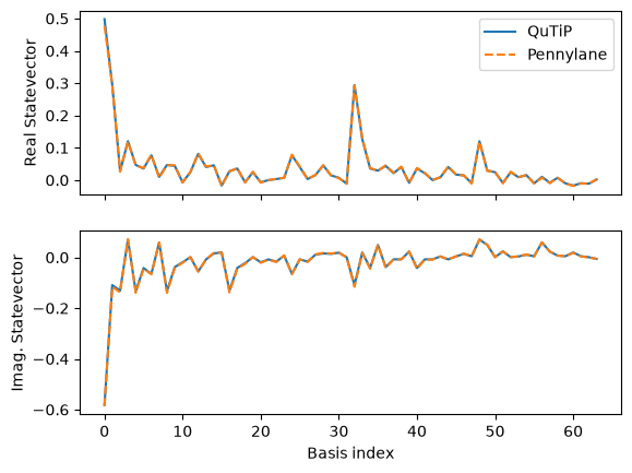
We find excellent argeement between the two methods.

fidelity = np.abs((np.conj(qutip_result) * pennylane_result).sum()) ** 2
print("Fidelity between methods is:", fidelity)

Fidelity between methods is: 0.9994373399826388

fig, axs = plt.subplots(nrows=2, sharex="col")

axs[0].plot(qutip_result.real, c="C0", label="QuTiP")
axs[0].plot(pennylane_result.real, ls="--", c="C1", label="Pennylane")
axs[0].legend()
axs[0].set_ylabel("Real Statevector")

axs[1].plot(qutip_result.imag, c="C0")
axs[1].plot(pennylane_result.imag, ls="--", c="C1")

axs[1].set_xlabel("Basis index")
axs[1].set_ylabel("Imag. Statevector")

plt.show()