Quantum Simulation Environment (QSE)#
Important
This project is under active development.
The Quantum Simulation Environment (QSE) is a flexible, modular, high-level Python library designed to decouple the essence of the quantum simulation problem from the technicalities of the backend software/hardware.
        ---
config:
  layout: tidy-tree

---
mindmap
   root((QSE))
      Qbits
         Qbit
         Cell
      Calculator
         Pulser
         MyQLM
         Qutip
      Utils
         Magnetic
         Signals
      lattices
         2D
         3D
      Visualise
Architectural Overview#
QSE organizes these concerns into modular components. The user interacts primarily
with the Qbits and Lattices to frame the problem, then attaches a Calculator.
Core Components#
1. Framing the System (Qbits)#
Qbits class represents the spatial setup, where you define the “What.”.
It is a collection of quantum degrees of freedom defined by their coordinates.
Instead of thinking about qubits as abstract indices in a register, you treat
them as physical entities with coordinates.
Arbitrary Coordinates: Place qubits exactly where you need them.
Lattice Generation: Quickly build 2D/3D grids (Square, Kagome, Triangular, etc.).
2. Solving the Problem (Calculator)#
The Calculator is a high-level wrapper. It defines the interaction between the
quantum degrees of freedom represented by the Qbits. Once Qbits are defined,
you “attach” them to a calculator. The calculator translates your physical setup
into the specific language required by the backend (e.g., Pulser’s pulses or QuTiP’s Hamiltonians).
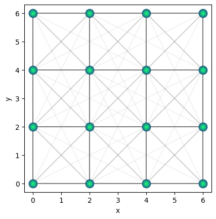
Quick Start: Defining a Lattice#
This example shows how easily a physical system on a lattice can be defined without any backend specific code.
import qse

# 1. Frame the problem: Create a 4x4 square lattice
qsqr = qse.lattices.square(
   lattice_spacing=2.0,
   repeats_x=4, repeats_y=4)

# 2. Visualise the lattice
qsqr.draw(radius=5.0)

# 3. Choose your backend calculator
# calc = qse.calc.Pulser(...)
# calc.qbits = qsqr # attach the system
Qbits#
Qbit is the smallest class that represents just one qubit. Qbits is the primary class that represents a collection of qubits.
It can be instantiated by providing a list of coordinates, or as an empty class.
See the Qbits examples for more details.
Calculator#
Calculators are high level wrappers that let us offload the quantum problem to several backends. Currently the list of backends supported are following, and they largely support analog quantum simulation.
        graph LR
    subgraph Framing [Problem Framing]
        Lattices --> Qbits
        Utils --> Qbits
    end

    subgraph Interface [The Connection]
        Qbits --- Calculator
    end

    subgraph Execution [Backend Execution]
        Calculator ---> Pulser
        Calculator ---> MyQLM
        Calculator ---> Qutip
    end
🎯 The Philosophy: Separation of Concerns#
The core value of QSE is the strict separation between Problem Framing and Problem Execution
Phase |
Responsibility |
User Focus |
|---|---|---|
Problem Framing |
|
Defining geometry, positions, and quantum degrees of freedom. |
Backend Execution |
|
Handling SDK-specific syntax, hardware constraints, and simulators. |
Why this matters:
Backend Agnostic: Frame your problem once; simulate it on Pulser, myQLM, or QuTiP just by switching one line of code.
No More “Jargon”: You don’t need to learn the specific pulse sequences or gate-level syntax of every vendor to get started. You focus on the lattice and the physics.
Reproducibility: Your problem definition remains a “clean” representation of the physical model, making it easier to share and verify across different research groups.
📍Position-Dependent Quantum Degrees of Freedom#
Unlike standard gate-based frameworks where qubits are abstract entities in a register, QSE treats qubits as physical objects with coordinates. This is crucial for simulations where the interaction strength between qubits is a function of their spatial separation.
Why Positions Matter#
In many physical implementations of quantum simulators—such as Rydberg Atom Arrays or Trapped Ions—the Hamiltonian of the system is governed by the distance \(R_{ij}=|{\bf R}_i - {\bf R}_j|\) between qubits \(i\) and \(j\):
In QSE, you don’t manually calculate these interaction terms. By defining the spatial degrees of freedom (the coordinates), QSE allows the backend calculators to automatically derive the physics based on the geometry you’ve framed.
The Mapping Process#
Define Geometry: You place qubits in a 1D, 2D, or 3D arrangement.
Assign Degrees of Freedom: Each qubit is assigned quantum properties (e.g., ground and Rydberg states).
Automatic Interaction Mapping: The
Calculatoruses the spatial data to build the interaction matrix (e.g., \(\frac{1}{r^6}\) or \(\frac {1}{r^3}\) scaling) specific to that backend’s hardware logic.
Status & Contribution#
QSE is currently under active development (TRL 7-8). This project was initially developed and supported by the HPCQS project and is currently supported by the QEX project. We are focused on expanding our calculator suite to support more backends and post-processing tools.
Target Users: Scientific researchers in quantum optimization and many-body physics.
Source Code: GitHub Repository
Contributing: See our Contribution Guide.
Tip
By keeping the problem definition independent of the backend, QSE ensures that the computational workflow remains portable even as the quantum hardware landscape changes.