Preparing Z-Orderings

In this notebook we explore the phase diagram of the Rydberg system and prepare several Z-ordering states.

See https://arxiv.org/pdf/1707.04344 for more details.

import matplotlib.pyplot as plt
import numpy as np

import qse

Computing the phase diagram

Recall the Rydberg Hamiltonian: $\( H = \frac{\hbar \Omega}{2} \sum_i X_i - \hbar \delta \sum_i N_i + \sum_{i<j} \frac{C_6}{r_{ij}^6}N_i N_j \)\( Suppose \)\Omega=0\(, and consider a \)1D\( chain with lattice spacing \)a\( (\)r_i=ia\(), then the Hamiltonian reads: \)\( H = - \hbar \delta \sum_i N_i + \frac{C_6}{a^6} \sum_{i<j} \frac{N_i N_j}{(i-j)^6} \)\( Note that in this case the Hamiltonian is diagonal and hence it is easy to compute the ground-state phase diagram. For \)\delta \le 0\( the Ground state contains zero excitations, thus we consider only \)\delta>0$.

n_atoms = 7
basis = qse.magnetic.get_basis(n_atoms)

interaction_term = np.zeros(basis.shape[0])

for c, b in enumerate(basis):
    for i in range(n_atoms - 1):
        for j in range(i + 1, n_atoms):
            if b[i] and b[j]:
                interaction_term[c] += 1.0 / (i - j) ** 6

c6 = 5420158.53  # (rad/µs)(µm)**6
interaction_term *= c6

spacings, dx = np.linspace(2, 20, 140, retstep=True)
energies = np.zeros_like(spacings)
phases = np.zeros_like(spacings, dtype=int)

delta = 2 * np.pi  # (rad/µs)
detuning = -delta * basis.sum(1)

for i, a in enumerate(spacings):
    energy = detuning + interaction_term / a**6
    energies[i] = np.min(energy)
    phases[i] = np.argmin(energy)

for s in np.unique(phases):
    inds = np.where(phases == s)[0]
    print(
        1 * basis[s],
        f"Spacing range: {spacings[inds[0]]:.2f}-{spacings[inds[-1]]:.2f} (µm)",
    )
    plt.plot(
        spacings[inds], energies[inds], label="".join(str(1 * b) for b in basis[s])
    )
    if not np.isclose(spacings[inds[-1]], spacings[-1]):
        plt.axvline(x=spacings[inds[-1]] + 0.5 * dx, c="k", ls="--", alpha=0.5)

plt.xlabel("Lattice spacing (µm)")
plt.ylabel("Ground state energy (rad/µs)")

plt.legend()

plt.show()

[1 0 0 0 0 0 1] Spacing range: 2.00-3.55 (µm)
[1 0 0 1 0 0 1] Spacing range: 3.68-5.76 (µm)
[1 0 1 0 1 0 1] Spacing range: 5.88-10.94 (µm)
[1 1 1 1 1 1 1] Spacing range: 11.06-20.00 (µm)

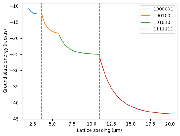
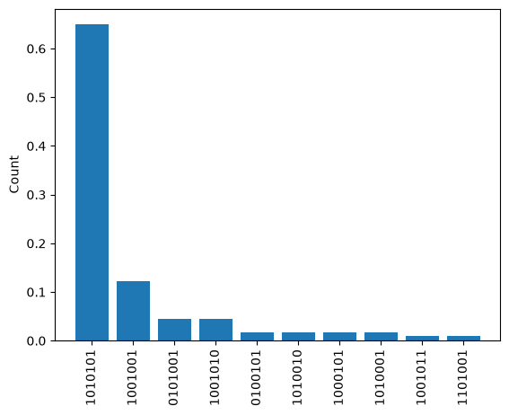
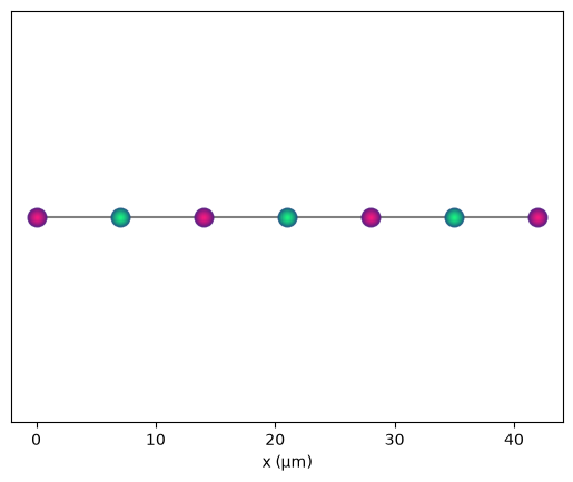
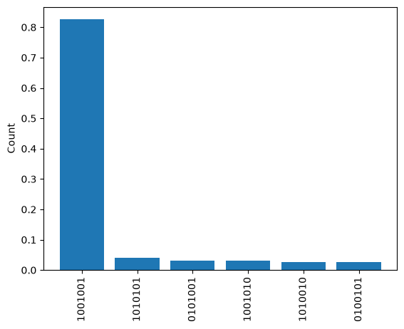
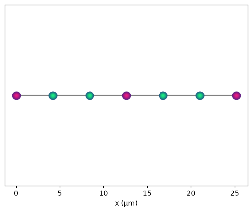
We see that for a lattice spacing of 3.68-5.76 (µm) we get a Z3 ordering (every 3 atoms are excited) while for a lattice spacing of 5.88-10.94 (µm) we get a Z2 ordering (every 2 atoms are excited). Let’s try and prepare both phases with an adiabatic pulse.

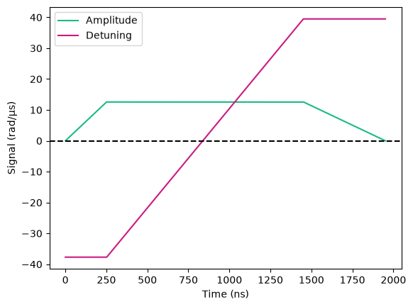
Adiabatic preparation

omega_max = 2.0 * 2 * np.pi  # rad/µs

delta_0 = -3 * omega_max  # rad/µs
delta_f = (2 * np.pi) * delta  # rad/µs

t_rise = 252  # ns
t_fall = 500  # ns
t_sweep = 1200  # ns

amplitude = qse.Signals()
amplitude += qse.Signal(np.linspace(0.0, omega_max, t_rise))
amplitude += qse.Signal([omega_max], t_sweep)
amplitude += qse.Signal(np.linspace(omega_max, 0.0, t_fall))

detuning = qse.Signals()
detuning += qse.Signal([delta_0], t_rise)
detuning += qse.Signal(np.linspace(delta_0, delta_f, t_sweep))
detuning += qse.Signal([delta_f], t_fall)

# Check both signals have the same duration
assert amplitude.duration == detuning.duration

fig = qse.vis.draw_amp_and_det(amplitude, detuning, "ns", "rad/µs")

for spacing in [7.0, 4.2]:
    qbits = qse.lattices.chain(spacing, n_atoms)

    pcalc = qse.calc.Pulser(
        qbits=qbits, amplitude=amplitude, detuning=detuning, wtimes=False
    )
    pcalc.build_sequence()
    pcalc.calculate(False)

    probs = (np.conj(pcalc.statevector) * pcalc.statevector).real

    p_dict = {"".join(str(1 * s) for s in basis[i]): p for i, p in enumerate(probs)}
    p_dict = {w: p_dict[w] for w in sorted(p_dict, key=p_dict.get, reverse=True)}

    fig = qse.vis.bar(p_dict, cutoff=0.01)
    qbits.draw(radius="nearest", units="µm", colouring=basis[np.argmax(probs)])

/home/runner/work/qse/qse/qse/qbits.py:1231: UserWarning: 1D system passed, adding a y axis.
  warnings.warn("1D system passed, adding a y axis.")
/home/runner/work/qse/qse/qse/qbits.py:1231: UserWarning: 1D system passed, adding a y axis.
  warnings.warn("1D system passed, adding a y axis.")