Quantum Adiabatic Pulses

Here we prepare a ground state of a Hamiltonian using an adiabatic pulse. See the adiabatic theory notebook for more details on the adiabatic theorem.

Recall the Rydberg Hamiltonian is

\[ H = \frac{\hbar \Omega(t)}{2} \sum_i X_i - \hbar \delta(t) \sum_i N_i + \sum_{i<j} \frac{C_6}{r_{ij}^6}N_i N_j \]

where \(\Omega\) is the Rabi frequency, \(\delta\) is the detuning, \(C_6\) is a device specific constant and \(r_{ij}\) is the distance between qubits \(i\) and \(j\).

We will choose the signals so that the initial Hamiltonian will be

\[ H_i = - \hbar \delta_i \sum_i N_i + \sum_{i<j} \frac{C_6}{r_{ij}^6}N_i N_j \]

by choosing a suitably negative value for \(\delta_i\) we ensure the ground state of the \(H_i\) is the all \(0\) state, which is the state we start in.

We will choose the signals so that the final Hamiltonian will be

\[ H_f = \frac{\hbar \Omega_f}{2} \sum_i X_i + \sum_{i<j} \frac{C_6}{r_{ij}^6}N_i N_j \]

and this is the Hamiltonian’s whose ground state we want to prepare.

import qse
import matplotlib.pyplot as plt
import numpy as np

delta_initial = -2.0
omega_final = 2.0

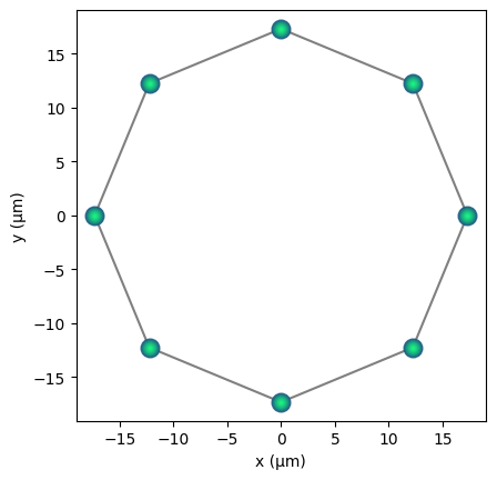
r_b = qse.calc.blockade_radius(omega_final * 0.5)
qbits = qse.lattices.ring(r_b, 8)
qbits.draw(radius="nearest", units="µm")

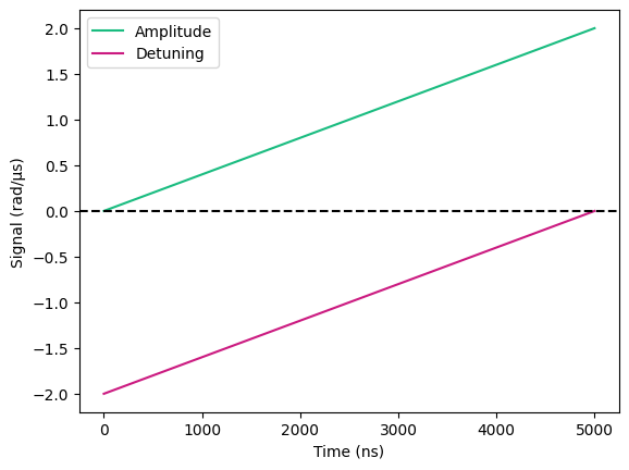
duration = 5000  # ns
amplitude = qse.Signal(np.linspace(0, omega_final, duration))
detuning = qse.Signal(np.linspace(delta_initial, 0, duration))

fig = qse.vis.draw_amp_and_det(amplitude, detuning, "ns", "rad/µs")
plt.show()

calc = qse.calc.Qutip(qbits, amplitude, detuning)

# We get the initial and final hamiltonians
h_i = calc.get_hamiltonian(amplitude[0], detuning[0])
h_f = calc.get_hamiltonian(amplitude[-1], detuning[-1])

# We compute the expectations of both Hamiltonians
results = calc.calculate(e_ops=[h_i, h_f])

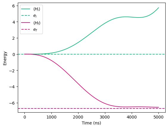
# Let's compute the groun-state energies of the initial and final hamiltonians
e_i = h_i.eigenenergies()[0]
e_f = h_f.eigenenergies()[0]

plt.plot(
    results["expectations"][:, 0], label=r"$\langle H_i \rangle$", c=qse.vis.qse_green
)
plt.axhline(e_i, ls="--", label=r"$e_i$", c=qse.vis.qse_green)

plt.plot(
    results["expectations"][:, 1], label=r"$\langle H_f \rangle$", c=qse.vis.qse_red
)
plt.axhline(e_f, ls="--", label=r"$e_f$", c=qse.vis.qse_red)

plt.ylabel("Energy")
plt.xlabel("Time (ns)")
plt.legend()
plt.show()

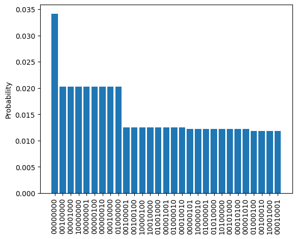
probs = np.real(np.conj(results["state"]) * results["state"]).flatten()
probs_dict = {f"{np.binary_repr(c, qbits.nqbits)}": p for c, p in enumerate(probs)}
probs_dict = {
    w: probs_dict[w] for w in sorted(probs_dict, key=probs_dict.get, reverse=True)
}
fig = qse.vis.bar(probs_dict, ylabel="Probability", cutoff=0.011)