Adiabatic Time Evolution#
Theory#
Suppose we have a Time-dependent Hamiltonian \(H(t)\) then the Schrödinger equation is $\( i\hbar \frac{d}{dt}|\psi(t)\rangle = H(t)|\psi(t)\rangle. \)\( We can write \)\( |\psi(t)\rangle = \sum_n c_n(t)|n(t)\rangle \)\( with \)\( H(t) |n(t)\rangle = e_n(t) |n(t)\rangle. \)$
The Adiabatic Theorem states that if a system is evolved by a slowly varying time dependent Hamiltonian (i.e. \(\dot H(t) \approx 0\)) and as long as the eigenenergies don’t become degenerate (i.e. \(e_n(t) - e_m(t) \ne 0\)) then we will have $\( |c_m(t)|^2 = |c_m(0)|^2.\)$ Thus as a consequence if the system is initially in the ground state of the Hamiltonian, if the evolution is adiabatic, it will remain in the Hamiltonian’s ground-state.
Single Qubit Example#
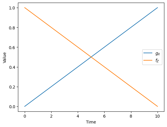
Consider the time dependent Hamiltonian $\( \begin{split} H(t) &= - f_Z(t) Z - g_X(t) X \\ f_Z(t) &= 1-t/T \\ g_X(t) &= t/T \\ \end{split} \)$ Note that at:
\(t=0\): \(H(0) = -Z \) and \(|0\rangle\) is the groundstate.
\(t=T\): \(H(T) = -X \) and \(|+\rangle\) is the groundstate.
The adiabatic theorem assues us that if we vary the Hamiltonian slowly enough (i.e. for a large value of \(T\)), the final evolved state will be the ground state of \(H(T)\) if we start in the ground state of \(H(0)\). Note that \(\dot H(t) = - (Z +X) /T\) which tends to zero for large values of \(T\), thus for large \(T\) the evolution will be adiabatic. In the cells below we start in the state \(|0\rangle\) and evolving slowly we will evolve to the state \(|+\rangle\).
import matplotlib.pyplot as plt
import numpy as np
import qutip as qp
duration = 10.0
sample_times = np.linspace(0, duration, 100)

pulse_up = lambda t: t / duration
pulse_dn = lambda t: 1.0 - t / duration


def get_ham(t):
    return -pulse_dn(t) * qp.sigmaz() - pulse_up(t) * qp.sigmax()
plt.plot(sample_times, pulse_up(sample_times), label="$g_X$")
plt.plot(sample_times, pulse_dn(sample_times), label="$f_Z$")
plt.xlabel("Time")
plt.ylabel("Value")
plt.legend()
plt.show()
initial_state = qp.fock(2)
states = qp.sesolve(
    get_ham, initial_state, sample_times, e_ops=[qp.sigmaz(), qp.sigmax()]
)
plt.plot(states.e_data[0], label="<Z>")
plt.plot(states.e_data[1], label="<X>")
plt.xlabel("Time")
plt.ylabel("Expectation Value")

plt.legend()
plt.show()
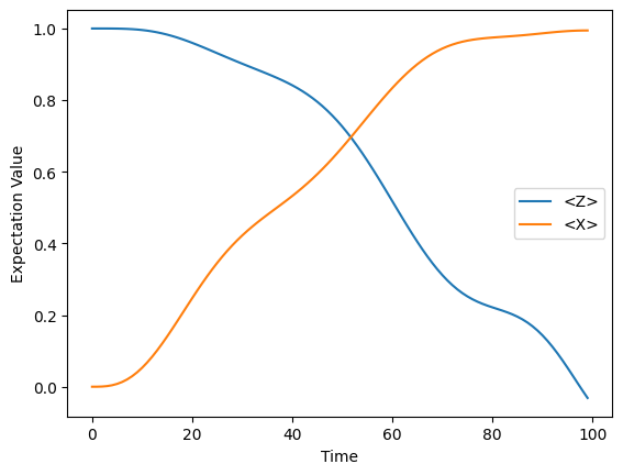
We see that initially \(\langle Z \rangle=1\) (since we start in the state \(|0\rangle\)) but after the evolution we have \(\langle x\rangle=1\) which shows we have correctly evolved to the state \(|+\rangle\).