Calculation Example

The following tutorial shows how to use qse to run a calculation. We use pulser here for the backend.

import numpy as np
import qse

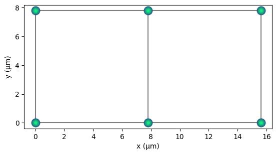
Create a 2D square lattice

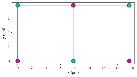
We generate the qbits object that represents a 2D lattice, keeping the lattice spacing a bit below the blockade radius keeps the nearest neighbours antiferromagnetic.

omega_max = 2.0 * 2 * np.pi  # rad/µs
rabi_frequency = omega_max / 2.0  # rad/µs

blockade_radius = qse.calc.blockade_radius(rabi_frequency)
q2d = qse.lattices.square(
    lattice_spacing=0.8 * blockade_radius, repeats_x=3, repeats_y=2
)

print(f"Blockade radius: {blockade_radius:.2f} µm")
q2d.draw(radius="nearest", units="µm")

Blockade radius: 9.76 µm

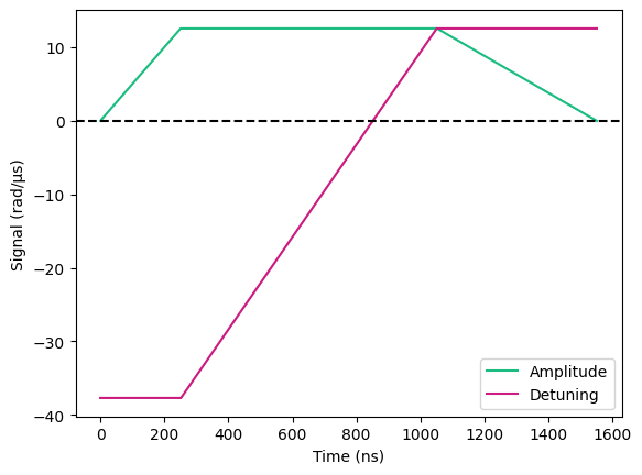
Create the hamiltonian

delta_0 = -6 * rabi_frequency  # ns
delta_f = 2 * rabi_frequency  # ns
t_rise = 252  # ns
t_fall = 500  # ns
t_sweep = int((delta_f - delta_0) / (2 * np.pi * 10) * 1000)  # ns

amplitude_afm = qse.Signals()
amplitude_afm += qse.Signal(np.linspace(0.0, omega_max, t_rise))
amplitude_afm += qse.Signal([omega_max], t_sweep)
amplitude_afm += qse.Signal(np.linspace(omega_max, 0.0, t_fall))

fig = amplitude_afm.draw("ns", "rad/µs", "Amplitude")

detuning_afm = qse.Signals()
detuning_afm += qse.Signal([delta_0], t_rise)
detuning_afm += qse.Signal(np.linspace(delta_0, delta_f, t_sweep))
detuning_afm += qse.Signal([delta_f], t_fall)

fig = detuning_afm.draw("ns", "rad/µs", "Detuning")

# Check both signals have the same duration
assert amplitude_afm.duration == detuning_afm.duration

Set up the calculator and run the job

pcalc = qse.calc.Pulser(qbits=q2d, amplitude=amplitude_afm, detuning=detuning_afm)
pcalc.build_sequence()
pcalc.calculate()

10.1%. Run time:   0.00s. Est. time left: 00:00:00:00

20.0%. Run time:   0.01s. Est. time left: 00:00:00:00

30.0%. Run time:   0.01s. Est. time left: 00:00:00:00

40.0%. Run time:   0.01s. Est. time left: 00:00:00:00

50.0%. Run time:   0.01s. Est. time left: 00:00:00:00

60.1%. Run time:   0.02s. Est. time left: 00:00:00:00

70.0%. Run time:   0.02s. Est. time left: 00:00:00:00

80.0%. Run time:   0.02s. Est. time left: 00:00:00:00

90.0%. Run time:   0.03s. Est. time left: 00:00:00:00

100.0%. Run time:   0.03s. Est. time left: 00:00:00:00

Total run time:   0.03s
time in compute and simulation = 0.09529709815979004 s.

Sample the result

count = pcalc.results.sample_final_state(N_samples=1000)
# Let's order by measurement frequency
count = {w: count[w] for w in sorted(count, key=count.get, reverse=True)}
fig = qse.bar(count, cutoff=10)

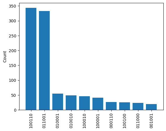
The states 011001 and 100110 are the most prevalent, we can visualise them using the colouring parameter in draw. We see that they correspond to anti-ferromagnetic orderings.

q2d.draw(radius="nearest", colouring="011001", units="µm")

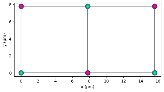
q2d.draw(radius="nearest", colouring="100110", units="µm")

Version

qse.utils.print_environment()

Python version: 3.12.13
qse version: 1.1.5