Simulating the SSH model

Here we simulate the SSH model using the Pulser backend. We follow the work of De Léséleuc et al. in “Observation of a symmetry-protected topological phase of interacting bosons with Rydberg atoms” (available also on arxiv).

Using a Microwave channel, the interaction Hamiltonian is given by

\[H = \sum_{i=1}^N \sum_{j<i} C_{ij} (\sigma_i^+ \sigma_j^- + \sigma_i^- \sigma_j^+)\]

where \(C_{ij} = \frac{C_3(1-3\cos^2\theta_{ij})}{R_{ij}^3}\). Here \(R_{ij}\) is the distance between qubits \(i\) and \(j\), \(R_{ij}=|\textbf{x}_i-\textbf{x}_j|\), and \(\theta_{ij}\) is the angle between \(\textbf{x}_i-\textbf{x}_j\) and the magnetic field. See the Pulser docs for more information.

By appropriate choice of the qubit geometry we can approximate the SSH model for hard bosons. For example, when $\( \theta_{ij} = \cos^{-1}\sqrt{1/3}\)$ there will be no interaction between qubits \(i\) and \(j\). We use this to model the SSH model below.

import qse
import numpy as np
import matplotlib.pyplot as plt

angle = np.arccos(np.sqrt(1.0 / 3.0)) * 180 / np.pi
print(f"Angle is: {angle:.2f} degrees")

Angle is: 54.74 degrees

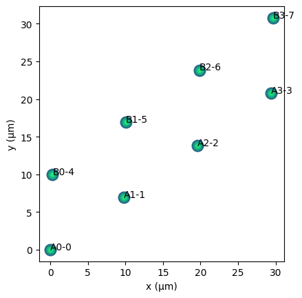
We create two chains of qubits, A and B. By rotating them by the angle above, there will be no interactions between qubits on the same chain.

lattice_spacing = 12
repeats = 4

qbits1 = qse.lattices.chain(lattice_spacing=lattice_spacing, repeats=repeats)
qbits1.labels = [f"A{i}-{i}" for i in range(repeats)]
qbits1.add_dim()  # Make 2D

qbits2 = qse.lattices.chain(lattice_spacing=lattice_spacing, repeats=repeats)
qbits2.labels = [f"B{i}-{i+repeats}" for i in range(repeats)]
qbits2.add_dim()
qbits2.translate((lattice_spacing * 0.5, 8))

qbits_ssh = qbits1 + qbits2
qbits_ssh.rotate(
    90 - angle
)  # by rotating to this angle interactions in the A & B chains will cancel.

qbits_ssh.draw(show_labels=True, units="µm")

We can verify that there are no interactions in the same chain by computing the couplings between qubits.

magnetic_field = np.array(
    [0.0, 1.0, 0.0]
)  # We need to define the field in 3D for the calculator.
c3 = 3700


def compute_hamilton_coef(i, j):
    """Compute the hamiltonian coefficient between qubits i & j."""
    r = qbits_ssh.positions[i] - qbits_ssh.positions[j]
    d = np.linalg.norm(r)
    r /= d
    cos_theta = np.dot(r, magnetic_field[:2])
    return c3 * (1 - 3 * cos_theta**2) / d**3


couplings = [
    [compute_hamilton_coef(i, j) for j in range(i + 1, qbits_ssh.nqbits)]
    for i in range(qbits_ssh.nqbits - 1)
]
couplings = [j for i in couplings for j in i]
coupling_mat = np.zeros((qbits_ssh.nqbits, qbits_ssh.nqbits))
coupling_mat[np.triu_indices(qbits_ssh.nqbits, 1)] = couplings
couplings
for i in range(1, qbits_ssh.nqbits):
    print(f"Coupling between qbits 0 & {i}:", coupling_mat[0, i])

Coupling between qbits 0 & 1: -4.754427304529029e-16
Coupling between qbits 0 & 2: -5.943034130661286e-17
Coupling between qbits 0 & 3: 0.0
Coupling between qbits 0 & 4: -7.391286573549234
Coupling between qbits 0 & 5: -0.5880494737584242
Coupling between qbits 0 & 6: -0.09525640675644509
Coupling between qbits 0 & 7: -0.026269374219942052

# Let's visualize the couplings
bonds = np.abs(coupling_mat)
bonds /= np.max(bonds)
qbits_ssh.draw(show_labels=True, units="µm")
for i in range(0, qbits_ssh.nqbits - 1):
    for j in range(i + 1, qbits_ssh.nqbits):
        xs_ij = qbits_ssh.positions[[i, j]]
        plt.plot(xs_ij[:, 0], xs_ij[:, 1], c="k", alpha=bonds[i, j], zorder=-1)

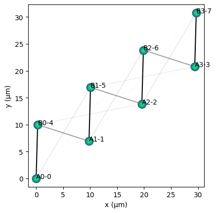
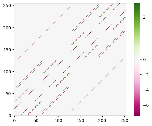
Thus we see that there are no couplings between qubits in the same chain, and hence we have a SSH model. Finally we can visualize the Hamiltonian.

pcalc_ssh = qse.calc.Pulser(
    qbits=qbits_ssh,
    amplitude=qse.Signal([0.0], 10),
    detuning=qse.Signal([0.0], 10),
    channel="mw_global",
    magnetic_field=magnetic_field,
)
pcalc_ssh.build_sequence()
pcalc_ssh.calculate()

10.0%. Run time:   0.00s. Est. time left: 00:00:00:00

20.0%. Run time:   0.00s. Est. time left: 00:00:00:00

30.0%. Run time:   0.00s. Est. time left: 00:00:00:00

40.0%. Run time:   0.00s. Est. time left: 00:00:00:00

50.0%. Run time:   0.00s. Est. time left: 00:00:00:00

60.0%. Run time:   0.00s. Est. time left: 00:00:00:00

70.0%. Run time:   0.00s. Est. time left: 00:00:00:00

80.0%. Run time:   0.00s. Est. time left: 00:00:00:00

90.0%. Run time:   0.01s. Est. time left: 00:00:00:00

100.0%. Run time:   0.01s. Est. time left: 00:00:00:00

Total run time:   0.01s
time in compute and simulation = 0.0682525634765625 s.

ham = pcalc_ssh.sim.get_hamiltonian(1).full()
fig = qse.visualise.view_matrix(ham.real, vcenter=0.0)

Version

qse.utils.print_environment()

Python version: 3.12.13
qse version: 1.1.5