Lecture 9: NISQ Algorithms I

Warning

These lecture notes are a work in progress and are not a replacement for watching the lecture video, it’s intended to be a supplementary reading after watching the lecture.

Focus of Lecture

Learning Outcomes

• What is the NISQ era?

• Why do we need NISQ algorithms?

• Example of NISQ algorithm: Variational Quantum Eigensolver (VQE)

Contents

• NISQ Era

• Classical optimisation

• Expectation Values

• VQE

• VQE Ansatzes

• Introduction to Hamiltonians

• VQE for chemistry

The NISQ Era

Drawbacks of early quantum algorithms

Implementing algorithms like Shor’s or Grover’s requires:

• Large amounts of qubits

• Long circuits

• Error correction (to be robust in the presence of noise), further increasing the number of required qubits.

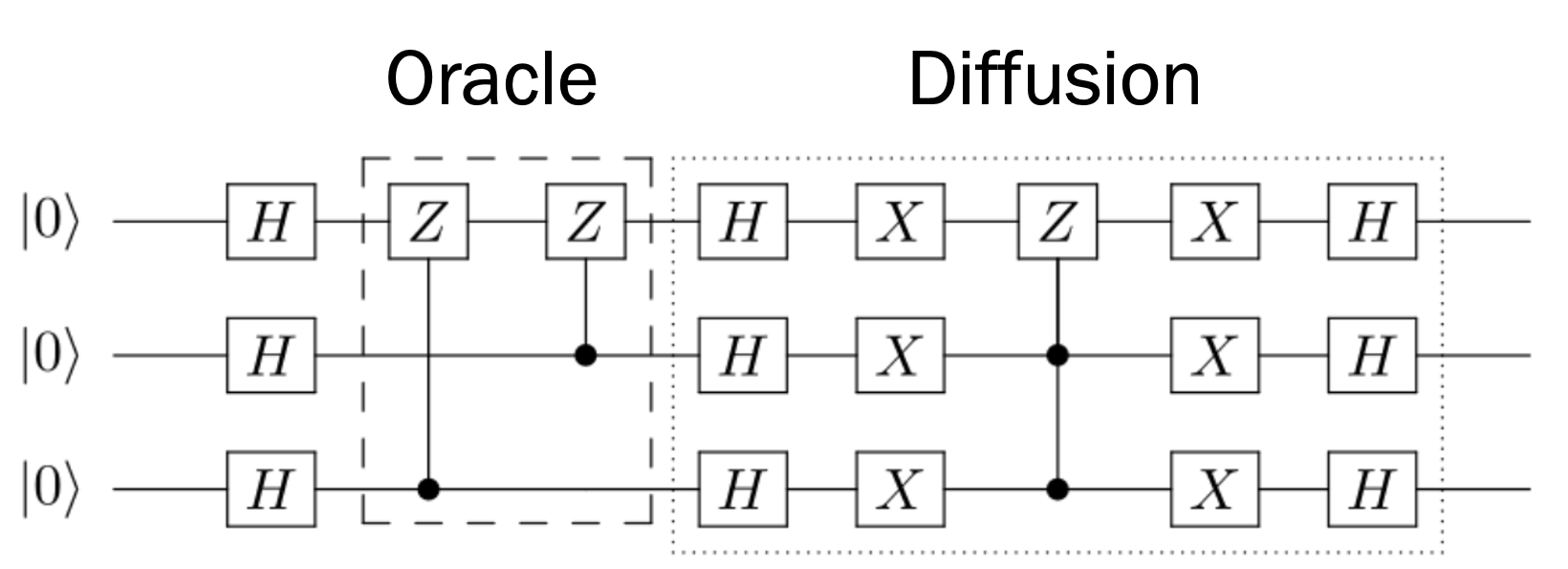
Fig. 68 Grover’s circuit requires many gates, which becomes infeasible on current quantum computers when we scale to larger instances.

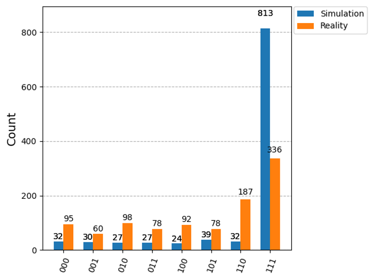
Fig. 69 Noise in the circuit leads to a loss of the expected output distribution, as shown here in the difference between ideal simulation and noisy reality. The more gates we have, the more noise is introduced.

Variational Quantum Algorithms

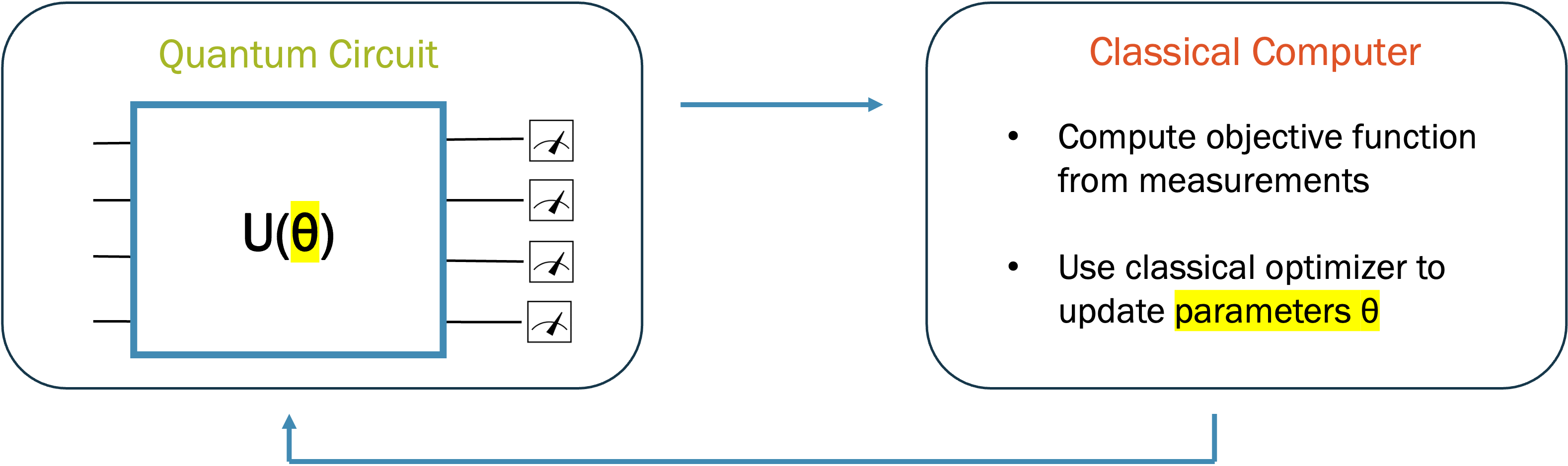
Fig. 70 Variational quantum algorithms use classical optimisation to find the best parameters for a quantum circuit.

Classical optimisation

Given a cost function \(f(x)\), find the input \(x\) that makes \(f\) as small as possible:

\[ x^* = \underset{x}{\arg\min}\; f(x) \]

• \(x\) can be a single number or a list of many parameters.

• We can usually evaluate \(f(x)\) for any chosen \(x\), but we can’t see the whole function at once.

• So we search iteratively: start from a guess, evaluate, improve the guess, repeat.

• Stop when \(f\) stops decreasing (convergence).

Hiker analogy

Think of a hiker in thick fog trying to reach the lowest point of a valley. They can only measure the height where they stand, so they try a few nearby steps and keep moving downhill.

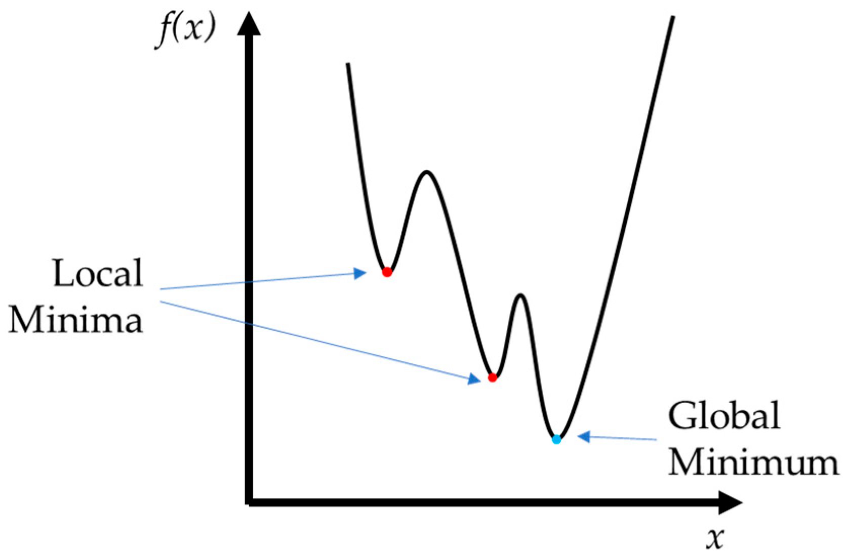
Fig. 71 Classical optimisation can get stuck in local minima, where the function is lower than all nearby points, but not the lowest point overall (the global minimum).

How does an optimiser improve its guess?

Gradient-based

The gradient \(\nabla f\) points uphill, so step the opposite way:

\[ x_{\text{new}} = x - \eta\,\nabla f(x) \]

• \(\eta\) is the step size (learning rate)

• Too large: overshoots the minimum

• Too small: very slow progress

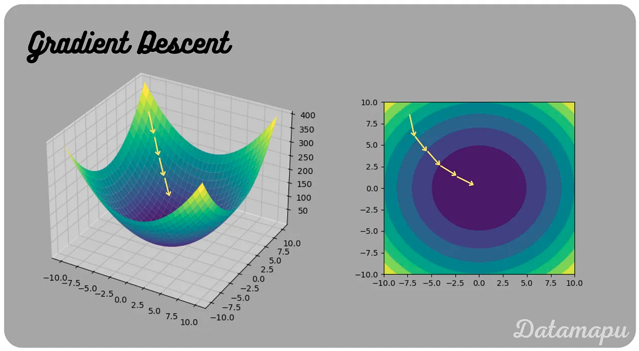
Fig. 72 Gradient descent repeatedly steps in the direction of steepest decrease. The step size \(\eta\) controls how far each step goes.

Gradient-free

• Only compare values of \(f\) at several trial points and move towards the better ones

• e.g. Nelder-Mead, COBYLA

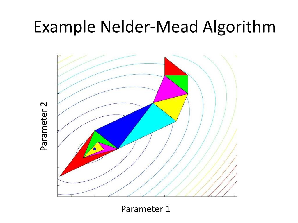
Fig. 73 The Nelder-Mead method evaluates \(f\) at the corners of a simplex (a triangle in two dimensions), then reflects, expands or shrinks it towards better values.

Things that can go wrong

• Local minima: the optimiser settles in a valley that isn’t the lowest one

• Flat regions: the gradient is almost zero, so progress stalls

• Noisy evaluations: if \(f(x)\) is only known approximately, comparisons and gradients become unreliable

• Cost per evaluation: methods that need fewer evaluations are preferred when each one is expensive

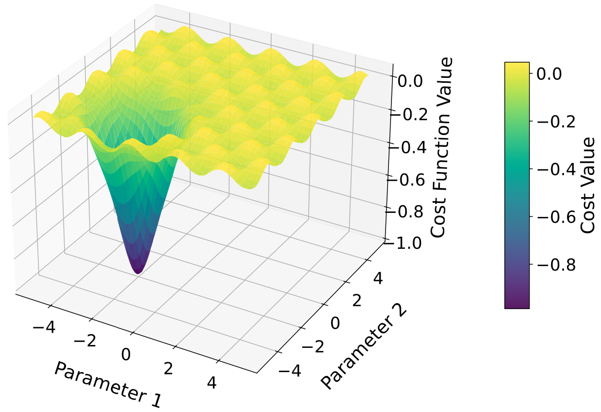
Fig. 74 A barren plateau: a region where the cost function is almost flat, so the gradient is close to zero and the optimiser has no useful direction to follow. Source: https://arxiv.org/pdf/2511.22861

NISQ Algorithms on Real Hardware

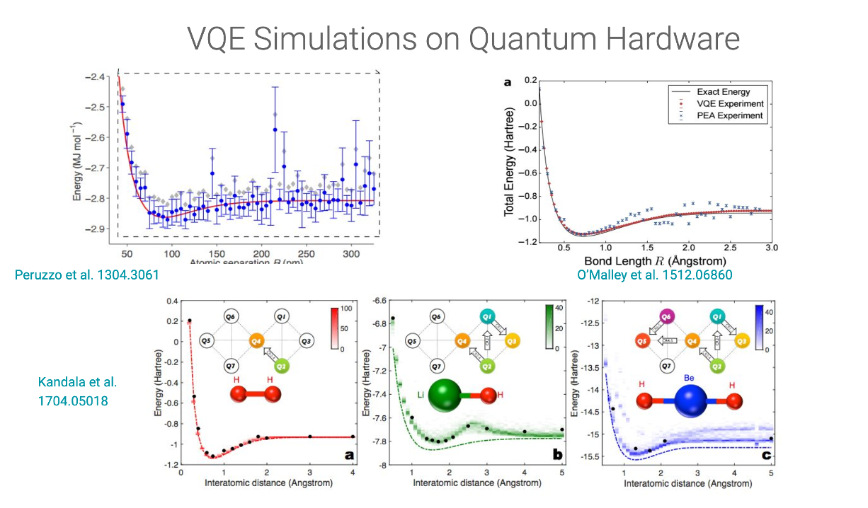
Fig. 75 Variational quantum algorithms (e.g. VQE, the variational quantum eigensolver) have already been run on real quantum hardware.

Expectation Values

First some recap on expectation values. A single measurement gives one random outcome, but if we repeat the experiment many times, the average outcome is well-defined and predictable. For an observable represented by a Hermitian operator \(\hat{O}\) and a state \(|\psi\rangle\), the expectation value is

\[ \langle \hat{O} \rangle = \langle\psi|\hat{O}|\psi\rangle \]

This is the average result you’d get measuring \(\hat{O}\) on many identically prepared copies of \(|\psi\rangle\). Recall that individual measurement outcomes are eigenvalues of \(\hat{O}\), denoted \(\lambda_i\). Hence we can equivalently calculate the average as a sum over all these outcomes weighted by probability:

\[ \langle \hat{O} \rangle = \sum_i \lambda_i \, P(\lambda_i)= \sum_i \lambda_i |\langle \lambda_i|\psi\rangle|^2 \]

where \(|\lambda_i \rangle\) are the eigenvectors of \(\hat{O}\) and \(P(\lambda_i)\) is the probability of measuring \(\lambda_i\).

Expectation value of Z

Suppose we wish to measure the expectation of \(Z\) for single qubits state \(|\psi\rangle\). Recall that states \(\color{blue} |0\rangle\) and \(\color{red} |1\rangle\) are eigenstates of \(Z\) with eigenvalues \(\color{blue}+1\) and \(\color{red}-1\)

\[ Z\color{blue} |0\rangle \color{black} = \color{blue} +|0\rangle\color{black} \qquad Z \color{red} |1\rangle \color{black} = \color{red}-|1\rangle \]

The expected value of \(Z\) is simply:

\[\langle \psi|Z|\psi\rangle = \sum_i \lambda_i \, P(\lambda_i) = \color{blue}+\color{black} P(\color{blue}+1\color{black})\color{red}-\color{black}P(\color{red}-1\color{black}) \]

We know from the Born rule the probability of each outcome is:

\[ P(\color{blue}+1\color{black}) = |\color{blue}\langle 0| \color{black}\psi\rangle|^2 \qquad P(\color{red}-1\color{black}) = |\color{red}\langle 1|\color{black}\psi\rangle|^2 \]

• On a simulator we can compute the Born rule probabilities exactly.

• On a real machine we can only make measurements of 0 or 1 for each qubit.

On hardware to estimate the expectation value of \(Z\) for a state we must run the circuit (that prepares the state) many times and average.

We run the circuit \(N\) times (\(N\) is called the number of shots) and record:

• \(N_0\): the number of \(0\)’s measured

• \(N_1\): the number of \(1\)’s measured

Then we can estimate the probabilities

\[ P(+1) \approx N_0/N \qquad P(-1) \approx N_1/N \]

and

\[\langle \psi|Z|\psi\rangle\approx \frac{N_0-N_1}{N}\]

Expectation value of X & Y

How do we measure the expectation value of \(X\)?

The eigenvalues and eigenstates of \(X\) are:

• \(+1\) for \(|+\rangle=(|0\rangle+|1\rangle)/\sqrt{2}\)

• \(-1\) for \(|-\rangle=(|0\rangle-|1\rangle)/\sqrt{2}\)

We know

\[\begin{split} \begin{split} P(+1) &= |\langle +|\psi\rangle|^2\\ P(-1) &= |\langle -|\psi\rangle|^2\\ \end{split} \end{split}\]

but note

\[\begin{split} \begin{split} |+\rangle &= H|0\rangle \\ |-\rangle &= H|1\rangle \\ \end{split} \end{split}\]

Thus

\[\begin{split} \begin{split} P(+1) &= |\langle 0|H^\dagger|\psi\rangle|^2=|\langle 0|H|\psi\rangle|^2\\ P(-1) &= |\langle 1|H^\dagger|\psi\rangle|^2= |\langle 1|H|\psi\rangle|^2\\ \end{split} \end{split}\]

Therefore to measure \(\langle\psi|X|\psi\rangle\)

• 1. Prepare the state

• 2. Apply a Hadamard gate

• 3. Measure whether the qubit is in state 0 or 1

Repeating steps 1, 2 and 3 for \(N\) shots we can use

\[\langle\psi|X|\psi\rangle\approx \frac{N_0-N_1}{N}\]

For the expectation value of \(Y\), the eigenvalues and eigenstates of \(Y\) are:

• \(+1\) for \(|i+\rangle=(|0\rangle+i|1\rangle)/\sqrt{2}\)

• \(-1\) for \(|i-\rangle=(|0\rangle-i|1\rangle)/\sqrt{2}\)

using

\[\begin{split} \begin{split} |i+\rangle &= SH|0\rangle \\ |i-\rangle &= SH|1\rangle \\ \end{split} \end{split}\]

where \(S\) is the phase gate

\[\begin{split}S=\sqrt{Z}= \begin{pmatrix} 1 & 0\\0 & i\\ \end{pmatrix} \end{split}\]

we get

\[\begin{split} \begin{split} P(+1) &= |\langle 0|H^\dagger S^\dagger|\psi\rangle|^2=|\langle 0|H S^\dagger|\psi\rangle|^2\\ P(-1) &= |\langle 1|H^\dagger S^\dagger|\psi\rangle|^2= |\langle 1|H S^\dagger|\psi\rangle|^2\\ \end{split} \end{split}\]

Therefore to measure \(\langle\psi|Y|\psi\rangle\)

• 1. Prepare the state

• 2. Apply a \(S^\dagger\) gate

• 3. Apply a Hadamard gate

• 4. Measure whether the qubit is in state 0 or 1

Repeating steps 1, 2 and 3 for \(N\) shots we can use

\[\langle\psi|Y|\psi\rangle\approx \frac{N_0-N_1}{N}\]

Summary of single Qubit Expectation values

Thus to measure

• \(X\) we apply a \(H\) gate

• \(Y\) we apply a \(S^\dagger\) gate then a \(H\) gate

• \(Z\) we don’t need to add extra gates

When measuring \(X\) or \(Y\) the addition of the extra gates ensures that we are measuring in the correct basis.

We execute the circuit for \(N\) shots and estimate the expectation as

\[\frac{N_0-N_1}{N}\]

where

• \(N_0\) is the number of times we measure \(0\)

• \(N_1\) is the number of times we measure \(1\)

Expectation Values of Multiple Qubits

To measure multiple qubit expectation values:

• Add any necessary additional gates to measure in correct basis

• Execute the circuit \(N\) times and record the bitstrings of the measured qubits \(x\)

• The expectation value is then:

\[\frac{\sum_x N_x P_x}{N}\]

• where \(N_x\) is the number of times bitstring \(x\) was measured

• \(P_x\) is the parity of bitstring \(x\) which is +1 when there’s an even number of \(1\)’s and -1 when there’s an odd number.

  • \(P_{101}=1\)

  • \(P_{10011}=-1\)

Variational Quantum Eigensolver

Concept of VQE

Why the ground state matters

In physics the ground state is very important. It determines a system’s stable configuration and low-energy properties (e.g. a molecule’s bond length, reactivity, stability).

        flowchart LR
    A["Ansatz (parameterized circuit)"]:::red --> B["Measure ⟨H⟩"]
    B --> C["Classical optimizer"]
    C -->|"Update parameters"| A
    C --> D["Ground state energy ≈ min⟨H⟩"]

    classDef red fill:#f4cccc,stroke:#cc0000,stroke-width:1px,color:#000;
    

• Parameterized quantum circuit (ansatz) to prepare trial state

• Measure expectation value of Hamiltonian with respect to this state

• Optimise circuit parameters classically to minimise energy to find approximate ground state

What does “ansatz” mean?

Ansatz is German for “approach”. In physics/maths it means an educated guess used as a starting point to solve a problem.

Variational Principle

1. If we guess a state \(|\psi(\theta)\rangle\), its energy \(E\) is at least the ground state energy \(E_0\):

   \[ E = {\langle\psi(\theta)|H|\psi(\theta)\rangle}\geq E_0 \]

2. We can get closer to the ground state energy by optimising the parameters \(\theta\) of the trial state \(|\psi(\theta)\rangle\).

3. A good choice of \(|\psi(\theta)\rangle\) can lead to higher accuracy.

This raises the question: how do we create the parametrised circuit (ansatz)?

VQE Ansatzes

Recap: Rotation Gates

The rotation gates are parameterised rotations about the X, Y, Z axes of the Bloch sphere.

Definition

\[\begin{split} \begin{split} R_X(\theta) &= \begin{pmatrix} \cos({\theta}/{2}) & -i\sin({\theta}/{2}) \\ -i\sin({\theta}/{2}) & \cos({\theta}/{2}) \end{pmatrix}\\ R_Y(\theta) &= \begin{pmatrix} \cos({\theta}/{2}) & -\sin({\theta}/{2}) \\ \sin({\theta}/{2}) & \cos({\theta}/{2}) \end{pmatrix}\\ R_Z(\theta) &= \begin{pmatrix} e^{-i\theta/2} & 0 \\ 0 & e^{i\theta/2} \end{pmatrix}\\ \end{split} \end{split}\]

Compact form

They can all be written in the form

\[ R_A(\theta) = \cos(\theta/2) I -i\sin(\theta/2) A \]

where \(I\) is the identity matrix and \(A\in\{X,Y,Z\}\).

Unlike the Pauli gates, which are strict \(180^{\circ}\) flips, these act as continuous tuning dials. For example:

\[R_X(\theta)|0\rangle=\cos(\theta/2)|0\rangle -i\sin(\theta/2) |1\rangle\]

Simple “hardware-efficient” ansatz

• Alternates layers of single-qubit rotations (\(R_y\)) with layers of CNOTs

• Native gates for superconducting qubits and trapped ions

• Rotations depend on tunable parameters \(\theta_i\)

• CNOTs generate the entanglement

• Repeating this block \(d\) times (“depth”) increases the expressibility of the ansatz

• However, greater depth means:

  • Longer circuits

  • More noise on real hardware

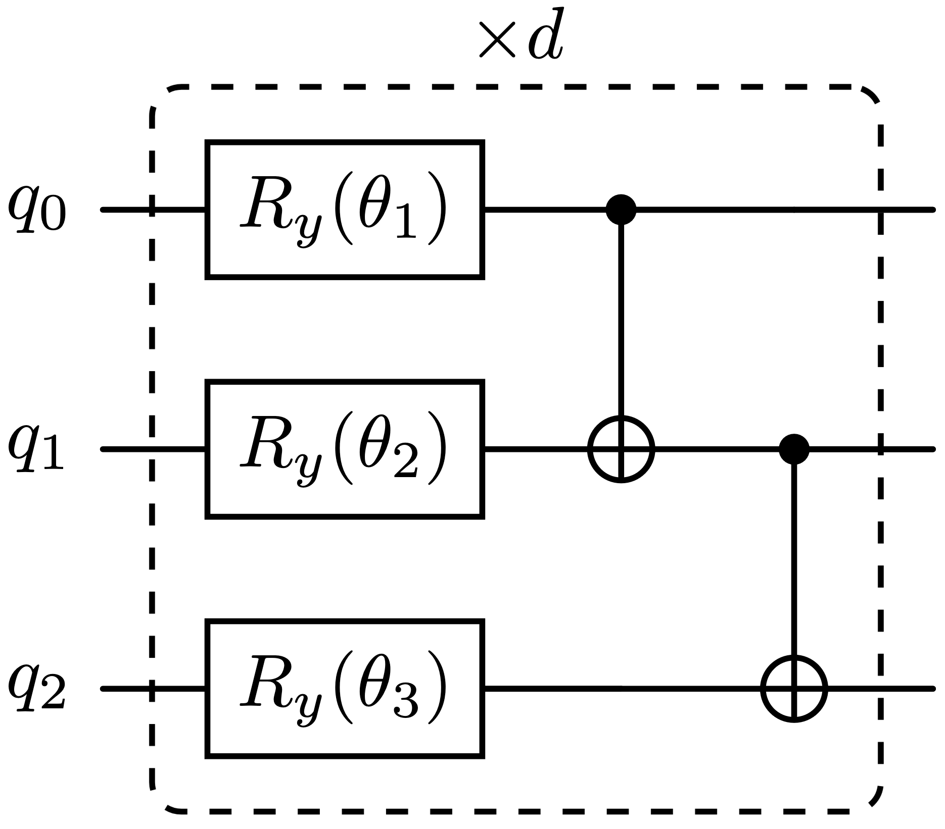
Fig. 76 A hardware-efficient ansatz: layers of parameterised single-qubit \(R_y\) rotations alternating with layers of CNOT gates.

Expressibility

Expressibility is the ability of a circuit to generate a wide variety of states. A more expressible circuit can represent a larger set of states.

Chemistry-inspired ansatz

• Built from physically motivated operators rather than generic gates

• Encodes knowledge of the structure of the problem into the circuit

• More parameter-efficient and physically meaningful for chemistry problems

• Typically requires deeper circuits to implement

• Example: Unitary Coupled Cluster (UCC) Ansatz:

Fig. 77 A Unitary Coupled Cluster (UCC) ansatz circuit.

VQE Workflow

        flowchart TD
    A["Problem"]:::red -->|"Encode"| B["Hamiltonian form H"]:::orange
    B --> VQE

    subgraph VQE["VQE"]
        direction TB
        C["Vary quantum state |ψ(θ)⟩ <br/>with parametrised circuit"]:::blue
        D["Classical optimiser<br/>updates θ so 𝐸 decreases"]:::blue
        C -->|"Measure 𝐸 = ⟨ψ(θ)|H|ψ(θ)⟩"| D
        D -->|"Update Parameters"| C
    end

    VQE -->|"repeat until 𝐸 converges"| E["Solution"]:::green

    style VQE fill:#e9d8fd,stroke:#6a3ea1,stroke-width:1px,opacity:1

    classDef red fill:#f4cccc,stroke:#cc0000,stroke-width:1px,color:#000;
    classDef orange fill:#fce5cd,stroke:#b45f06,stroke-width:1px,color:#000;
    classDef blue fill:#cfe2f3,stroke:#1155cc,stroke-width:1px,color:#000;
    classDef green fill:#d9ead3,stroke:#38761d,stroke-width:1px,color:#000;
    

1. Generate normalised ansatz state \(|\psi(\theta)\rangle\) on quantum computer

2. Measure \(E = \langle\psi(\theta)|H|\psi(\theta)\rangle\)

3. Optimise \(\theta\) on a classical computer so that \(E\) decreases

4. Repeat until \(E\) converges to obtain an approximate ground state

VQE on NISQ Hardware

Hybrid algorithm

• Quantum computer prepares parameterised trial state (ansatz) and measures the energy

• Classical optimiser updates parameters to minimise energy

• Loop repeats until convergence

Why it suits NISQ

• Classical optimiser reduces workload for QPU: only use quantum for the part that is inherently quantum

• Flexible ansatz can be tailored to hardware connectivity

Limitations

• Long circuits, many gates: decoherence and gate errors dominate

• Accuracy bar is high: to compete with classical methods

• Barren plateaux: gradients vanish exponentially with system size, stalling optimisation

• Measurement overhead: many circuit repetitions needed per energy evaluation, and per optimisation step

Introduction to Hamiltonians

In Quantum Physics the energy is represented by an operator, called the Hamiltonian, \(H\). The expected energy of a given state \(|\psi\rangle\) is the expectation value of the Hamiltonian

\[E=\langle \psi|H|\psi\rangle.\]

The ground state of a quantum system is the state with the lowest energy. To find the ground state we find the state that minimizes the expected Energy. The ground state is very important as it is the state of system at zero temperature (and at low temperatures the system will be at approximately the ground-state). Thus if we are interested in the properties of a molecule at room temperature, a starting place is to investigate the ground-state properties.

The Ising Model

Let’s look at a simple physics model to get a feel for Hamiltonians. We consider a single electron bound to an atom. Recall that electrons have a property called spin which can interact with external magnetic fields. The spin can be either up or down (or in a superposition of both). We’ll denote the up spin state as \(|0\rangle\) and the down spin state as \(|1\rangle\).

If a magnetic field, \(B\), is applied along the x-axis the Hamiltonian is

\[H=-BX\]

with ground state

\[|+\rangle=(|0\rangle+|1\rangle)/\sqrt 2.\]

Electrons can interact with each other via their spins. A two electron state is represented as \(|ij\rangle\), here the electron at atom 1 has spin \(i\) and the electron at atom 2 has spin \(j\). So for example \(|01\rangle\) would mean the electron at atom \(1\) has spin up and the electron at atom \(2\) has spin down.

A common way spins interact is through the Hamiltonian

\[H=- J Z \otimes Z =- J Z_1 Z_2\]

For this Hamiltonian

• If \(J>0\): The ground-states are \(\{|00\rangle, |11\rangle\}\), i.e. both electrons are aligned in spin

• If \(J<0\): The ground-states are \(\{|01\rangle, |10\rangle\}\), i.e. both electrons are anti-aligned in spin

Now let’s put both pieces together:

• A magnetic field in the x-axis

• Neighbouring interactions between electrons

For two qubits we get

\[H = -BX_0 - BX_1 - J Z_0 Z_1\]

This model is known as the Ising model, for \(n\) atoms (qubits) arranged in a chain it is

\[ H = -B \sum_{i=0}^{n-1}X_i - J \sum_{i=0}^{n-2} Z_i Z_{i+1} \]

where we note that the interactions are only between electrons on neighbouring atoms.

VQE for chemistry

In quantum chemistry we are interested in solving the electronic structure problem, this means to solve the Schrödinger equation for the electrons in a given molecule. This can given us information on a range of quantities including: a molecule’s bond length’smolecules, the energy required to remove an electron from a molecule or the structure of a molecule at low temperature.

It’s an amazing and surprising fact that many systems in both phsyics and chemistry can be described by Hamiltonians composed of Pauli operators. To give one example the Hamiltonian for a hydrogen molecule (two Hydrogen atoms) is approximately

\[\begin{split} \begin{split} H = &− 0.807 I + 0.175 Z_0 Z_2 + 0.169 Z_1Z_3 − 0.230 (Z_2 + Z_0) + 0.173 (Z_3 + Z_1) \\ &+ 0.045 (Y_0 Y_1 Y_2 Y_3 + X_0 X_1 Y_2 Y_3 ) + 0.045 (Y_0Y_1X_2X_3 + X_0 X_1 X_2X_3) \\ &+ 0.166 (X_0 Z_3 + Z_1Z_2) + 0.121 (Z_0 Z_1 + Z_2 Z_3) \end{split} \end{split}\]

Here the basis states are slightly different than before

• 0 represents spin up on atom 1

• 1 represents spin up on atom 2

• 2 represents spin down on atom 1

• 3 represents spin down on atom 2

Thus for example:

• \(|0000\rangle\) represents the state with no electrons

• \(|0111\rangle\) represents the state with one electron spin up on atom 1, and two electrons on atom 2 (spin up and down).

For computing the ground-state energy of molecules we can use the VQE workflow as previously described. We just have to add an extra step of mapping the molecule to the qubits of the quantum computer. We can do this by associating each molecular orbitas (a possible spatial configuration for an electron in the molecule) with two qubits:

• \(|00\rangle\) = empty orbital

• \(|01\rangle\) = one electron (spin down)

• \(|10\rangle\) = one electron (spin up)

• \(|11\rangle\) = two electrons (paired i.e. opposite spins)

When running the VQE for quantum chemistry we often benchmark our results against:

• Hartree-Fock (HF): An approximate way of solving the Schrödinger equation. It uses an average of the electron interactions. An efficient method but with limited accuracy.

• Full Configuration Interaction (FCI): An exact way of solving the Schrödinger equation. It considers all possible electron configurations. The computational cost of FCI scales exponentially with molecule size, so it can only be used for small molecules.