Lecture 4: First Quantum Algorithm

Warning

These lecture notes are a work in progress and are not a replacement for watching the lecture video, it’s intended to be a supplementary reading after watching the lecture.

Learning Outcomes

Learning Outcomes

• Understand what a quantum algorithm is and how it differs from a classical one.

• How a quantum algorithm is represented using quantum circuits.

• Study the Deutsch algorithm, one of the earliest quantum algorithms.

• Understand how quantum algorithms are programmed.

Algorithm: Definition

Algorithm

An algorithm is a set of instructions that solves a given problem.

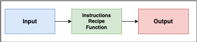
Fig. 5 Algorithm diagram.

• A classical algorithm is based on binary operations or the moving around of bits (0’s and 1’s).

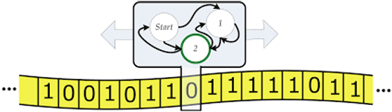
Fig. 6 Algorithm binary representation.

• A classical algorithm is always run on classical hardware.

Quantum Algorithm: Definition

Quantum Algorithm

A quantum algorithm is an algorithm that leverages quantum mechanics in terms of design and/or hardware.

Attention

Some algorithms are designed leveraging quantum mechanical properties, but run in a classical hardware.

Its basic unit of information is the qubit. It exhibits the following properties:

1. Superposition: A qubit can be in combination of \(\ket{0}\) and \(\ket{1}\) states.

2. Entanglement: Qubits can be correlated in ways that have no classical equivalent. Measuring the state of one qubit instantely tells us something about another.

3. Interference: A quantum algorithm can be designed so that the “wrong” answers interfere destructively and the right answers interfere constructively.

Superposition, Entanglement, Interference

1. Superposition

\[H\ket{0} = \frac{1}{\sqrt{2}}\ket{0} + \frac{1}{\sqrt{2}}\ket{1}\]

Superposition

The qubit is in both states at once — measuring gives 0 or 1, each with probability 1/2.

2. Entanglement

\[\frac{1}{\sqrt{2}}\ket{00} + \frac{1}{\sqrt{2}}\ket{11}\]

Entanglement

Measuring qubit 1 instantly fixes qubit 2’s outcome.

3. Interference

\[H H \ket{0} = \left(\tfrac{1}{2}+\tfrac{1}{2}\right)\ket{0} + \left(\tfrac{1}{2}-\tfrac{1}{2}\right)\ket{1} = \ket{0}\]

Interference

The \(\ket{1}\) amplitudes cancel (destructive), the \(\ket{0}\) amplitudes add (constructive).

Classical vs Quantum Algorithms

1. Basic unit of information

• Classical: Works with bits. Each bit is definitely either 0 or 1 at every point in time.

• Quantum: Works with qubits. Qubits can show superposition, entanglement and interference.

2. How states are processed

• Classical: to check N possibilities, a classical computer generally has to look at them one at time.

• Quantum: N qubits in superposition represent all \(2^{N}\) combinations of states simultaneously.

Attention

Even if quantum algorithms work with a superposition of states, measuring collapses the system to one result.

3. Gates

• Classical: Classical gates implement boolean logic functions on bitstrings.

• Quantum: Quantum gates implement linear transformations (represented by unitary matrices) on state vectors.

4. Reversibility

• Classical: most classical logic gates are irreversible. We can’t uniquely reconstruct the input from its output.

• Quantum: quantum gates must be reversible. This means they can always be run backward.

Attention

Reversibility of quantum gates is a hard mathematical constraint on how quantum circuits are built.

5. Algorithm output

• Classical: Algorithm output is deterministic in nature.

• Quantum: Measurement is probabilistic in nature.

6. Mathematical foundations

• Classical: Based on boolean algebra and discrete math. Bitstrings are transformed by logical operations.

• Quantum: Based on linear algebra over Hilbert spaces. Statevectors are transformed by unitary matrices.

Attention

Any classical algorithm can be represented and executed on a quantum computer.

Computational Complexity

• Computational complexity is the study of time and space resources required to solve computational problems.

• The big-O notation (\(O\)) is used to study the worst-case behaviour of specific algorithms.

• \(f(n)\) is in the class of functions \(O(g(n))\) means:

Big-O Notation

There exists constants \(c\) and \(n_0\) such that for all \(n>n_0\rightarrow f(n)<cg(n)\)

• In computational complexity, \(n\) can represent a wide variety of things, like the number of inputs, variables, qubits, gates, iterations…

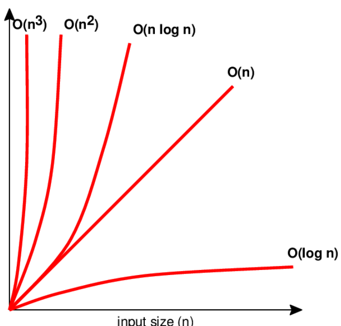
Fig. 7 Growth of common complexity classes.

• A simple sorting algorithm (e.g. bubble sort) is a good example of computing an algorithm’s complexity.

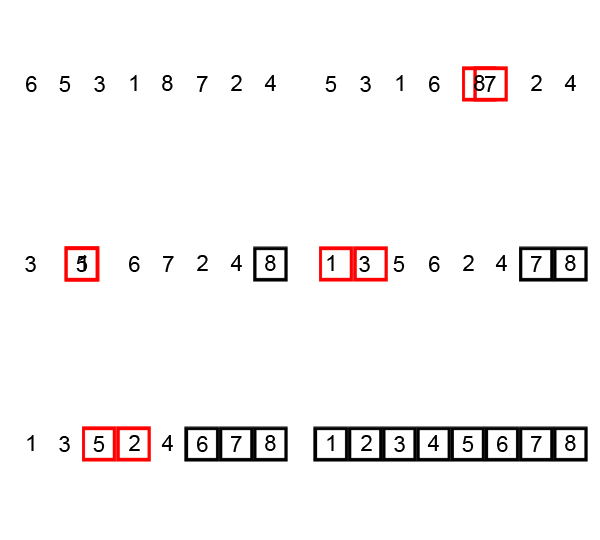
Fig. 8 Bubble sort algorithm animation. Source: commons.wikipedia.org

• The bubble sort is a simple (and inefficient) sorting algorithm.

• It steps through the list element by element, comparing adjacent elements and swapping their values if the order is not right.

• This means it has to do \((N-1) + (N-2) + \dots + 2 + 1 = \frac{N(N-1)}{2}=\frac{1}{2}(N^{2}-N)\) swaps in the worst case.

Attention

For large \(N\), the \(N^2\) term dominates, so bubble sort is said to have \(O(N^2)\) complexity.

Circuits

• In theoretical computer science a circuit is a model of computation in which input values go through a sequence of gates, each of which computes a function.

• Classical (quantum) algorithms can be implemented using complex sequences of classical (quantum) circuits.

• Circuits can be thought as an ordered sequence of operations, where each individual operation is a gate.

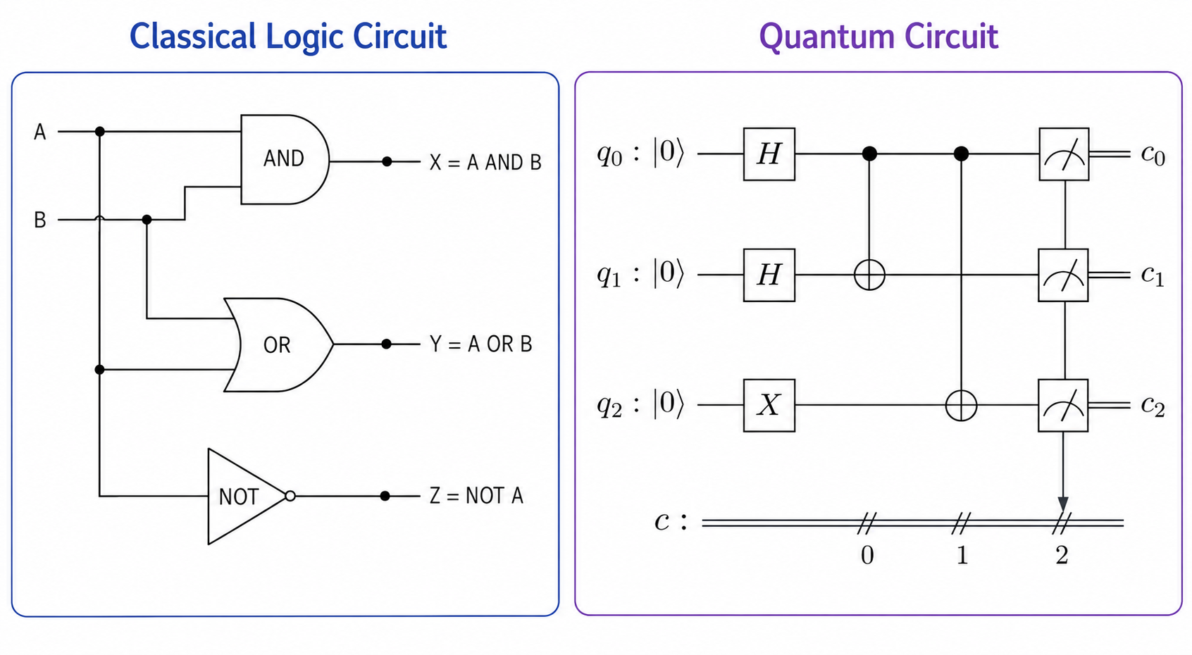
Fig. 9 Example of classical and quantum circuits.

Classical and Quantum Circuits: Differences and Similarities

1. Similarity: Gate ordering

• Both are partially ordered sequences of gates: independent gates can be reordered or run in parallel.

2. Difference: Gate timing

• Classical: Gate execution times are essentially uniform across gate types.

• Quantum: Gate execution times are not uniform. Different gates take different amounts of time to implement on real hardware.

3. Difference: Circuit depth

• Classical: Circuit depth is not as important as classical bits don’t suffer from decoherence.

• Quantum: Depth is critical, since qubits have a limited lifetime due to decoherence.

Quantum Circuits

• In a quantum circuit, wires represent qubits and gates represent operations on these qubits.

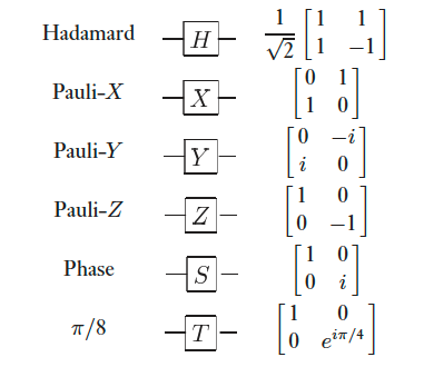
Fig. 10 Names, symbols and unitary matrices for common single qubit gates.

• Unless stated otherwise, qubits in a circuit are initialised to \(\ket{0}\) state.

• Circuits are read left to right. Gates to the left are applied first.

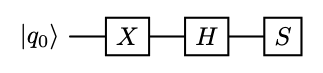
Fig. 11 Quantum circuit example.

\[\begin{split}\begin{aligned} SHX\ket{q_0} &= SHX\ket{0} = SH\ket{1}= \\ &= S\frac{1}{\sqrt{2}}\left(\ket{0}-\ket{1}\right) = \frac{1}{\sqrt{2}}\left(\ket{0}-i\ket{1}\right) \end{aligned}\end{split}\]

Multi-Qubit Circuits

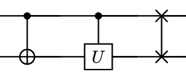
Fig. 12 Common two-qubit gates: CNOT, general controlled-U and SWAP gate.

• Multi-qubit states in circuits are usually written as \(\ket{q_0q_1\dots q_{n-1}}\) (big-endian ordering).

Attention

Some SDKs like Qiskit use little-endian ordering, which means that multi-qubit states are written as \(\ket{q_{n-1}\dots q_1\dots q_{0}}\). In all cases, however, \(q_0\) will be at the top when drawing the circuit.

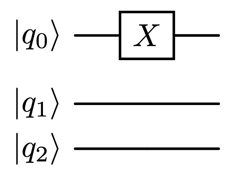
Fig. 13 Quantum circuit example to show big-endian little-endian differences.

Attention

The state of the circuit above would be \(\ket{001}\) in little-endian ordering and \(\ket{100}\) in big-endian ordering.

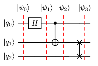
Fig. 14 3 qubit quantum circuit example.

\[\begin{split} \begin{aligned} \ket{\psi_0} &= \ket{000} \\[0.5em] \ket{\psi_1} &= (H_0\otimes I_1\otimes I_2)\,\ket{\psi_0} = \tfrac{1}{\sqrt{2}}(\ket{000}+\ket{100}) \\[0.5em] \ket{\psi_2} &= (\text{CNOT}_{01}\otimes I_2)\,\ket{\psi_1} = \tfrac{1}{\sqrt{2}}(\ket{000}+\ket{110}) \\[0.5em] \ket{\psi_3} &= (I_0\otimes \text{SWAP}_{12})\,\ket{\psi_2} = \tfrac{1}{\sqrt{2}}(\ket{000}+\ket{101}) \end{aligned} \end{split}\]

Measurement

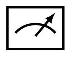
Fig. 15 Computational basis measurement symbol.

Attention

Even if measurement is drawn as a quantum gate, it is not. Measurement is not unitary. It is probabilistic and irreversible.

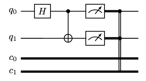
Fig. 16 Example of measurement with classical registers.

• The outcomes of measurements are written into a classical bit in the classical register.

• Classical registers enable conditional operations after mid-circuit measurements, applying quantum gates conditioned to the values in the classical register.

Attention

Sometimes all classical registers are drawn using just one double wire, or even not drawn at all.

Classical Circuit Example: The Half Adder

• The half adder is an example of a binary logical classical circuit.

• It takes two 1-bit inputs and produces:

  1. SUM: A XOR B.

  2. CARRY: A AND B.

• It is called “half” adder because it doesn’t account for a carry-in from previous stage.

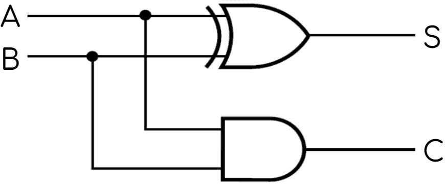
Fig. 17 Half adder circuit.

A	B	Sum	Carry
0	0	0	0
0	1	1	0
1	0	1	0
1	1	0	1

Half Adder

When we run an algorithm on a classical computer, it is made of a lot of logical circuits like the half-adder.

Quantum Circuit Example: The Half Adder

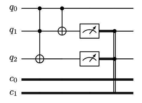
Fig. 18 Half adder quantum circuit.

• The Toffoli gate computes the carry operation, \(q_2 = A \cdot B\).

• The CNOT gate computes the sum, \(q_1 = A \oplus B\).

• Measuring \(q_1\), \(q_2\) reads out the sum and carry into the classical register.

Attention

This is just classical logic embedded reversibly into unitary gates, no superposition or interference is used. There’s no quantum speedup: it needs an extra ancilla qubit and offers no efficiency gain over a classical half adder.

Deutsch Problem

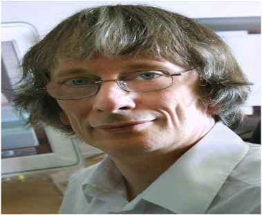
Fig. 19 David Deutsch.

• Given a black box \(f : \{0,1\} \rightarrow \{0,1\}\)

\[\begin{split}\begin{cases} f(0) = f(1) = 0 \\ f(0) = f(1) = 1 \end{cases} \Rightarrow \textcolor{green}{\textbf{Constant } f}\end{split}\]

\[\begin{split}\begin{cases} f(0) = 0,\ f(1) = 1 \\ f(0) = 1,\ f(1) = 0 \end{cases} \Rightarrow \textcolor{blue}{\textbf{Balanced } f}\end{split}\]

• Uses an oracle to determine if \(f\) is constant or balanced.

• Classically -> 2 queries.

• Deutsch algorithm -> 1 query.

• Early example of QC power (1985).

Quantum Parallelism

Quantum Parallelism

Quantum parallelism allows quantum computers to evaluate a function f(x) for different values of x simultaneously.

• For a binary function, it is possible to build a gate \(U_f\) that performs the transformation:

\[U_f\ket{x,y}=\ket{x,y\oplus f(x)}\]

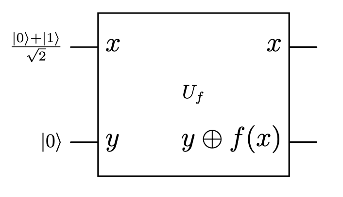
Fig. 20 Parallelism oracle example.

• Input state: \(\ket{\psi_0}=\frac{1}{\sqrt{2}}(\ket{0,0}+\ket{1,0})\)

• XOR gate (\(\oplus\)) truth table:

\(x\)	0	1	0	1
\(y\)	0	0	1	1
\(x\oplus y\)	0	1	1	0

\[U_f\ket{\psi_0}=\frac{1}{\sqrt{2}}(\ket{0,f(0)}+\ket{1,f(1)})\]

Attention

\(f(0)\), \(f(1)\) are evaluated simultaneously! But only one value is accessed per measurement.

Oracle

• For a 1-bit function there are only 4 possible oracles.

Constant f

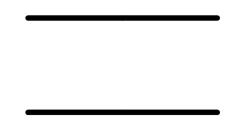
Fig. 21 \(f(x)=0\)

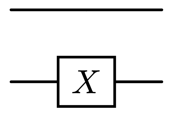
Fig. 22 \(f(x)=1\)

Balanced f

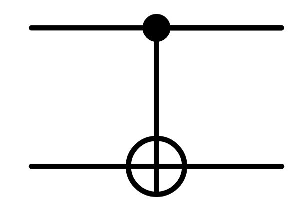
Fig. 23 \(f(x)=x\)

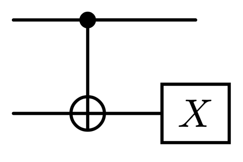
Fig. 24 \(f(x)=1-x\)

Deutsch Algorithm

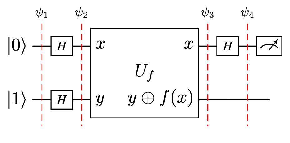
Fig. 25 Deutsch Algorithm.

1. Initial state.

2. Superposition generated using Hadamard gates.

3. Evaluate values f(x) using the oracle (parallelism).

4. Interference between states.

\[\ket{\psi_1}=\ket{0}\ket{1}\]

\[\ket{\psi_2}=\left(\frac{\ket{0}+\ket{1}}{\sqrt{2}}\right)\left(\frac{\ket{0}-\ket{1}}{\sqrt{2}}\right)\rightarrow\]

\[\ket{\psi_3}=\frac{1}{\sqrt{2}}\left((-1)^{f(0)}\ket{0}+(-1)^{f(1)}\ket{1}\right)\left(\frac{\ket{0}-\ket{1}}{\sqrt{2}}\right)\]

\[\ket{\psi_4}=\pm\ket{f(0)\oplus f(1)}\left(\frac{\ket{0}-\ket{1}}{\sqrt{2}}\right)\]

Deutsch Algorithm

Solves the problem in just one measurement!

Note

In order to get the state \(\ket{\psi_3}\), we used the fact that \(U_f\left[\ket{x}\left(\frac{\ket{0}-\ket{1}}{\sqrt{2}}\right)\right] = (-1)^{f(x)}\ket{x}\left(\frac{\ket{0}-\ket{1}}{\sqrt{2}}\right)\). Let’s see why:

\[U_f\left[\ket{x}\left(\frac{\ket{0}-\ket{1}}{\sqrt{2}}\right)\right] = \ket{x}\left[\frac{\ket{f(x)}-\ket{f(x)\oplus 1}}{\sqrt{2}}\right]\rightarrow\]

\[\begin{split}\rightarrow \left\{\begin{array}{c}\text{if } f(x)=0\rightarrow \ket{x}\left(\frac{\ket{0}-\ket{1}}{\sqrt{2}}\right) \\ \text{if } f(x)=1\rightarrow -\ket{x}\left(\frac{\ket{0}-\ket{1}}{\sqrt{2}}\right)\end{array}\right.\rightarrow\end{split}\]

\[\rightarrow U_f\left[\ket{x}\left(\frac{\ket{0}-\ket{1}}{\sqrt{2}}\right)\right] = (-1)^{f(x)}\ket{x}\left(\frac{\ket{0}-\ket{1}}{\sqrt{2}}\right)\]

Deutsch-Jozsa Algorithm

• If \(f\) is n-bit:

• Deutsch-Jozsa algorithm (1992) -> 1 query.

• Classically -> Can be up to \(2^{n-1}+1\) queries.

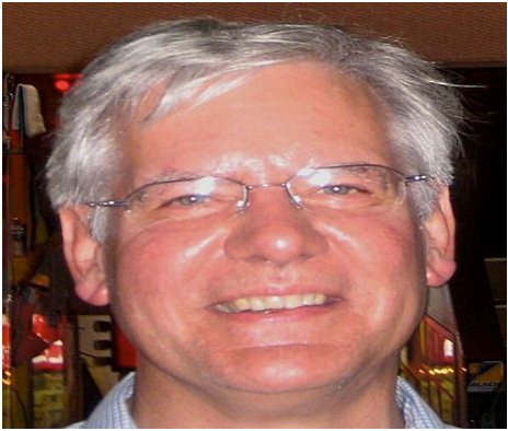
Fig. 26 Richard Jozsa.

• Looks like a big improvement but…

1. Deutsch problem has no known practical applications.

2. The method evaluating the function it’s different between the classical and quantum case.

3. If we use a classical probabilistic algorithm, we can drastically reduce the number of queries needed to solve the problem with high confidence.

Classical Programs

Classical Program

A classical computer program is a set of instructions in a programming language for a classical computer to execute.

• One can think of a classical computer program as a concrete implementation of a classical algorithm.

random_integer.py

import numpy as np
import matplotlib.pyplot as plt

samples = np.random.randint(16, size=1000)
values, counts = np.unique(samples, return_counts=True)

plt.bar(values, counts)
plt.xlabel("Value")
plt.ylabel("Count")
plt.show()

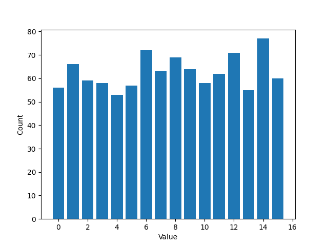
Fig. 27 Output of random_integer.py.

Quantum Programs

Quantum Program

A quantum program is a set of instructions in a programming language for a quantum computation.

Attention

A quantum program can be executed on a quantum computer or simulated in a quantum simulator.

Attention

A quantum program may be composed of one or more quantum circuits.

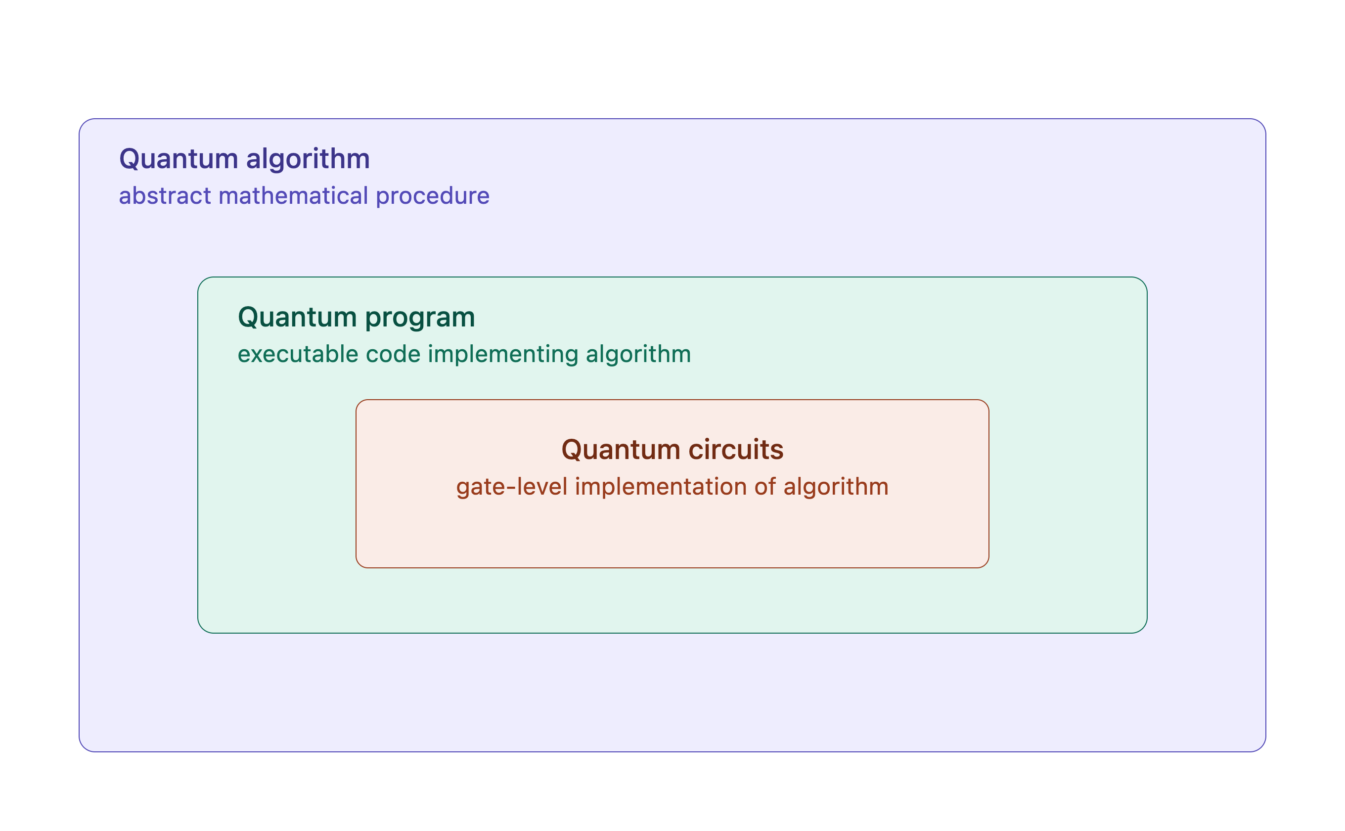
Fig. 28 Quantum algorithm, program and circuit hierarchy.

random_integer_quantum.py

import matplotlib.pyplot as plt
from qiskit import QuantumCircuit
from qiskit_aer import AerSimulator

qc = QuantumCircuit(4, 4)
qc.h(range(4))
qc.measure(range(4), range(4))

counts = AerSimulator().run(qc, shots=1000).result().get_counts()

values = [int(bitstring, 2) for bitstring in counts]
weights = list(counts.values())

plt.bar(values, weights)
plt.xlabel("Value")
plt.ylabel("Count")
plt.show()

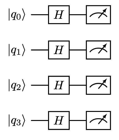
Fig. 29 Circuit of random_integer_quantum.py.

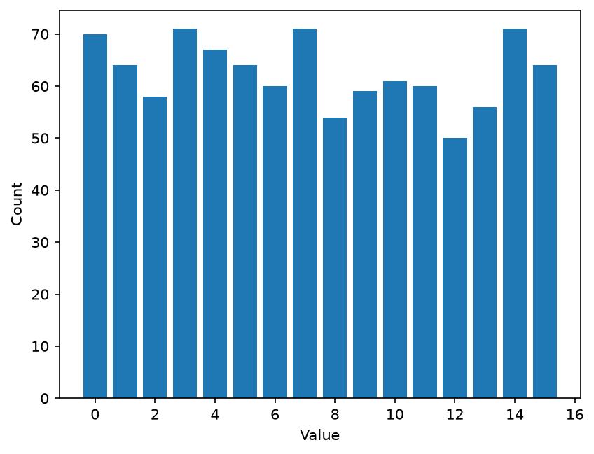
Fig. 30 Output of random_integer_quantum.py.

Quantum Simulators

Quantum Simulator

A quantum simulator is a classical system that reproduces the behaviour of a quantum computer.

• Running algorithms on real hardware is very expensive.

• Using quantum simulators allows us to look for bugs, prototype algorithms or do resource estimation before sending them to a real device.

• The number of amplitudes grows as \(2^n\), so simulating larger systems gets exponentially harder.

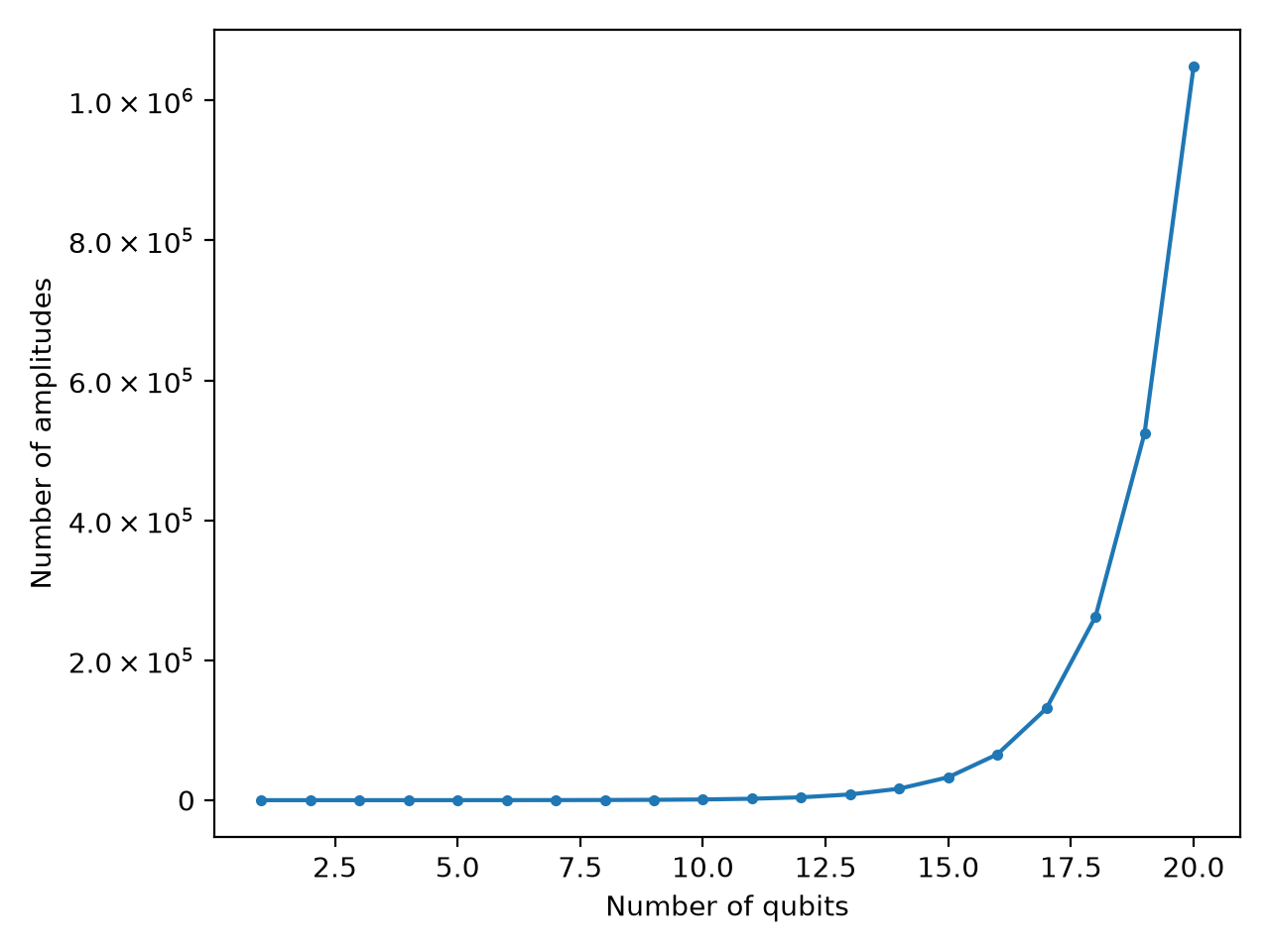
Fig. 31 Number of amplitudes vs. number of qubits.

Statevector Simulators

Statevector Simulator

A statevector simulator represents the full quantum state as a single complex vector of length \(2^n\).

• The statevector simulator is the default simulator in almost all SDKs.

• The number of quantum amplitudes grows exponentially with the number of qubits.

• Statevector simulation uses brute force to perform the simulation. It is the most exact, but among the most computationally expensive simulators.

• Simulating more than 40 qubits with a statevector simulator requires supercomputer-scale distributed memory.

Accesing Quantum Computing Systems

Quantum Stack

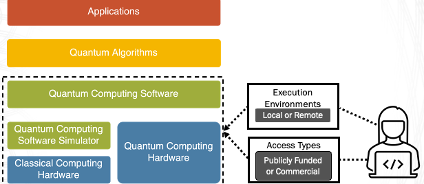
Fig. 32 The quantum computing stack.

• The user can interact with the software and hardware elements of the quantum stack in different ways.

• Quantum programs can be executed locally or remotely, and using commercial or publicly-funded systems.

Quantum Computing Software Simualtors (QCSS)

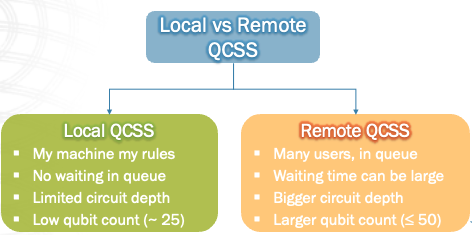
Fig. 33 Local and remote QCSS.

• QCSS can be installed locally on one’s laptop or workstation.

• Remote QCSS are installed on larger scale HPC facilities.

Accessing Quantum Computing Software Simulators

• Simulators can be roughly split into two categories: full-stack simulators bundled as a backend of a specific SDK, and standalone simulators used independently of any SDK.

Simulator	Language	Category	Notes
Qiskit Aer	C++	Full-stack	Qiskit’s backend; supports statevector, density-matrix, MPS and stabilizer methods
PennyLane Lightning	C++	Full-stack	PennyLane’s state-vector backend, with CPU, GPU and MPI variants
Cirq	Python	Full-stack	Google’s SDK; built-in cirq.Simulator state-vector simulator
ProjectQ	Python / C++	Full-stack	Open-source framework with a high-performance built-in simulator
Amazon Braket	Python	Full-stack	AWS Braket SDK’s local statevector / density-matrix simulators
Intel Quantum Simulator (IQS)	C++ / MPI	Standalone	Distributed-memory state-vector simulator, formerly qHiPSTER
Qulacs	C++ / Python	Standalone	Fast state-vector simulator with SIMD, OpenMP and GPU support
QuEST	C	Standalone	Multithreaded, distributed, GPU-accelerated statevector and density-matrix simulator
qsim	C++	Standalone	High-performance state-vector simulator, usable via Cirq or on its own
Stim	C++ / Python	Standalone	Very fast stabilizer-circuit simulator, built for QEC research
NVIDIA cuQuantum	C++ / Python (CUDA)	Standalone	GPU-accelerated libraries (cuStateVec, cuTensorNet) used as a backend by many simulators
MQT DDSIM	C++ / Python	Standalone	Decision-diagram based simulator from the Munich Quantum Toolkit
quimb	Python	Standalone	Tensor-network library used for large circuit simulation

Tightly-Integrated vs Heterogeneous Quantum Stacks

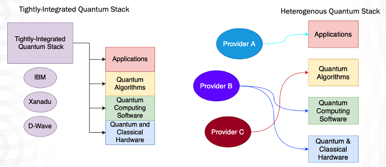
Fig. 34 Tightly-integrated vs heterogeneous quantum stack

• Tightly integrated quantum stacks are stacks in which the software layer and the quantum computing layer are developed by the same provider.

• Heterogeneous quantum stacks are stacks in which their elements are developed by different providers.

High-Level Quantum Software

• A quantum programming environment is a type of human-computer interface used to create programs to run on quantum computers or quantum software simulators.

• Once a quantum program is created, similar to classical programs, it can be compiled into instructions that your choice of hardware can understand and execute.

• Some quantum programming languages (QPLs) are standalone languages (e.g. Q#, Silq), while others are libraries/extensions added on top of an existing classical language.

• Most quantum programming libraries today are built on Python (e.g. Qiskit, PennyLane), though other languages are supported too, such as Julia (Yao.jl) or the C ++ (Intel SDK).

• Aside from generic quantum languages and libraries, there are also specialised languages and libraries designed and optimised for specific application domains, like quantum chemistry, QNLP and QML. For example, Tequila is geared towards solving problems in the quantum chemistry domain, while Lambeq represents sentence grammatical structure in the form of a quantum circuit: the sentence “John walks in the park” is deconstructed using diagrammatic methods and then represented as a quantum circuit, which can be used in NLP applications such as classification or sentiment analysis.

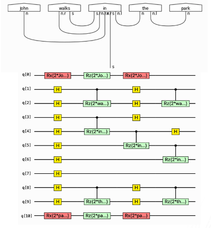
Fig. 35 Image example of lambeq library

Low-Level Quantum Software

• Low-level quantum software refers to intermediate representation (IR) languages that serve as an interface between many high-level quantum software languages and the target quantum computing hardware.

• In a similar way to classical programming, high-level languages are translated to an intermediate language, which is then used to apply the instructions to quantum hardware.

• One of the more common intermediate languages is OpenQASM. For example, a Bell state written in high-level Qiskit code compiles down to the equivalent OpenQASM circuit.

• Some consider these intermediate representations the equivalent to assembly in the classical programming world. They provide similar functionality: different high-level QPLs can be compiled to the same IR, which provides a mechanism to target different quantum systems with the same high-level code.