
Lecture 8: Early Quantum Algorithms III#
Warning
These lecture notes are a work in progress and are not a replacement for watching the lecture video, it’s intended to be a supplementary reading after watching the lecture.
Focus of Lecture#
After this lecture you should be able to:
Understand Grover’s Algorithm.
Have an intuition for the difference between quantum and classical random walks.
Grover’s Algorithm#
Grover’s algorithm is an algorithm for searching through an unstructed database. It ofters a quadratic speed-up over classical approaches.
Unstructured search#
We can formulate the search problem more formally as follows: Suppose we’re given a function
Our goal is to find a solution, which is a binary string \(x\in\{0,1\}^n\) for which \(f(x)=1\).
As an example consider the 2-bit function F given by the following table:
\(x\) |
\(F(x)\) |
|---|---|
00 |
0 |
01 |
0 |
10 |
1 |
11 |
0 |
This function has only one bitstring, 10, for which we get the output 1.
Our job is to find this bitstring 10 when we have access to the function as a circuit or a blackbox.
While this may seem abstract, in the real world searching through databases is a very common task.
Classically we can solve this by iterating through all \(x\) and evaluating \(f\) on each one and stopping when we find \(f(x)=1\). If there are \(N\) elements in the list and only one solution then on average we will have to evaluate \(N/2\) elements. Thus classically this problem is \(O(N)\).
Grover’s Operator#
For a database of size \(N=2^n\) we require \(n\) qubits. We define the oracle, \(O\), which performs the operation
thus if \(|x\rangle\) is a solution, \(O|x\rangle=-|x\rangle\).
We also define the phase shift which applies the follow transformation:
where here \(|0^n\rangle\) is the state with all \(n\) qubits in \(|0\rangle\), e.g. for \(n=4\), \(|0^4\rangle=|0000\rangle\). The phase shift corresponds to the following unitary:
where \(I\) is the identity matrix. To see this, note that it correctly transforms \(|0^n\rangle\rightarrow |0^n\rangle\) and for \(x\ne 0^n\), \(|x\rangle\rightarrow -|x\rangle\).
Grover’s operator consists in the following steps:
Apply the oracle \(O\)
Apply a Hadamard gate to each qubit
Apply the phase shift
Apply a Hadamard gate to each qubit
Steps 2-4 are called diffusion and can be combined together into unitary
where we have defined the uniform superposition state:
e.g. for \(n=2\), \(|\psi\rangle=\frac{1}{2}(|00\rangle+|01\rangle+|10\rangle+|11\rangle)\)
Thus we can define Grover’s operator, G, as
which comprises \(\color{red}\text{Diffusion}\) and an \(\color{blue}\text{Oracle}\).
Grover’s Circuit#
Grover’s algorithm consists in
Apply a Hadamard gate to each qubit (creating a uniform superposition state)
Apply Grover’s operator \(\sim\sqrt{N}\) times
Meaure the qubits
with a probability of at least \(1/2\) a solution will be measured.
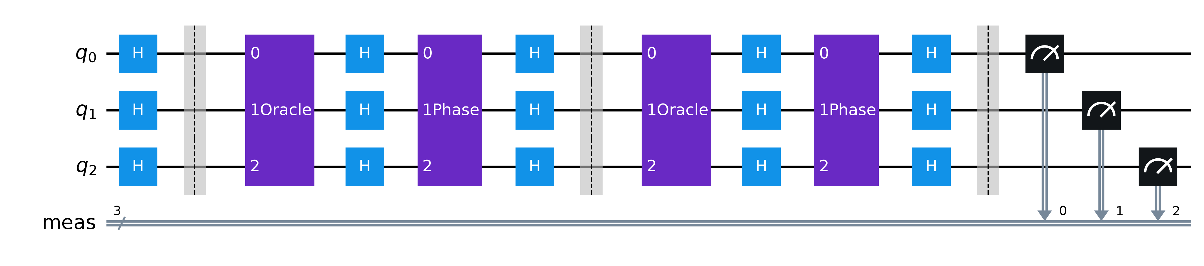
Fig. 61 Grover’s circuit for \(n=3\), here we apply Grover’s operator twice.#
Why does Grover’s algorithm work?#
We define \(M\) to be the number of solutions (i.e. values of \(x\) for which \(f(x)=1\)).
We define an equal superposition of solutions
where we some over all bit strings \(x\) which have \(f(x)=1\), and an equal superposition of non-solutions
Note that we can write the uniform superposition state \(|\psi\rangle\) in terms of these two states
where we have defined \(\phi=M / N\).
Consider a linear combination of \(|A_0\rangle\) and \(|A_1\rangle\)
note that the state the circuit is in before the first application of Grover’s application is \(|\psi\rangle\) and hence is in the form of \(|\alpha\rangle\).
If we apply Grover’s operator to \(|\alpha\rangle\) we get
Note that \(0 \le \phi \le 1\) and hence \(-1 \le 1-2\phi \le 1\), this means we can write
and hence
Thus using this new \(\theta\) variable we get
In terms of the coefficients \(a_0\) and \(a_1\), applying Grover’s operator to \(|\alpha\rangle\) results in the transformation
In the 2-D plane with \(|A_0\rangle\) being the x-axis and \(|A_1\rangle\) being the y-axis, this corresponds to an anti-clockwise rotation of angle \(\theta\).

Fig. 62 Applying Grover’s operator to state \(|\alpha\rangle\) results in an anti-clockwise rotation.#
Let’s suppose that the number of solutions \(M\) is small, then \(\phi=M/N\) must also be small. Thus we can approximate \(\phi(1-\phi)\approx \phi\) and hence \(\sin \theta = 2\sqrt{\phi(1-\phi)} \approx 2\sqrt{\phi}\). But if \(\phi\) is small then we can approximate \(\sin \theta\approx \theta\) and hence we end up with
Recall that the first step of Grover’s algorithm is to apply a Hadamard gate to each qubit, creating the uniform superposition state \(|\psi\rangle\), if \(M\) is small then \(|\psi\rangle\approx |A_0\rangle\). Thus we start very close to the \(|A_0\rangle\) state, recall that Grover’s operator rotates anticlockwise by angle \(\theta\), if we wish to end up near the \(|A_1\rangle\) we need to rotate by \(90\) degrees or \(\pi/2\) radians. Thus the number of rotations we require, \(k\), is
Thus we have derived the \(O(\sqrt N)\) scaling of Grover’s algorithm.
Classical Random Walks#
Classical random walks can be used to model:
The stock market (Economics)
The random motion of molecules (Chemistry)
Population dynamics (Biology)
For the simplest random walk we are restricted to move in a 1-dimensional line. At each time step we randomly take a step left or right with equal probability.
If we start at the origin where will we be after \(n\) steps? Let \(p_n(x)\) be the probability of being at position \(x\) after \(n\) steps.
After \(1\) step we either have taken a single step left or right, so the possible paths are L and R and hence:
\(p_1(-1)=1/2\)
\(p_1(1)=1/2\)
After \(2\) steps the possible paths are LL, LR, RL and RR and hence:
\(p_2(-2)=1/4\)
\(p_2(0)=1/2\)
\(p_2(2)=1/4\)
After \(3\) steps the possible paths are LLL, LLR, LRL, LRR, RLL, RLR, RRL and RRR and hence:
\(p_3(-3)=1/8\)
\(p_3(-1)=3/8\)
\(p_3(1)=3/8\)
\(p_3(3)=1/8\)
It can be shown that \(p_n(x)\) has the following properties
The mean is zero, \(\mu=\sum_x p_n(x) x=0\)
The variance is \(n\), \(\sigma^2=\sum_x p_n(x) (x-\mu)^2=n\)
Additionally when \(n\) is large the distribution tends towards a bell curve.
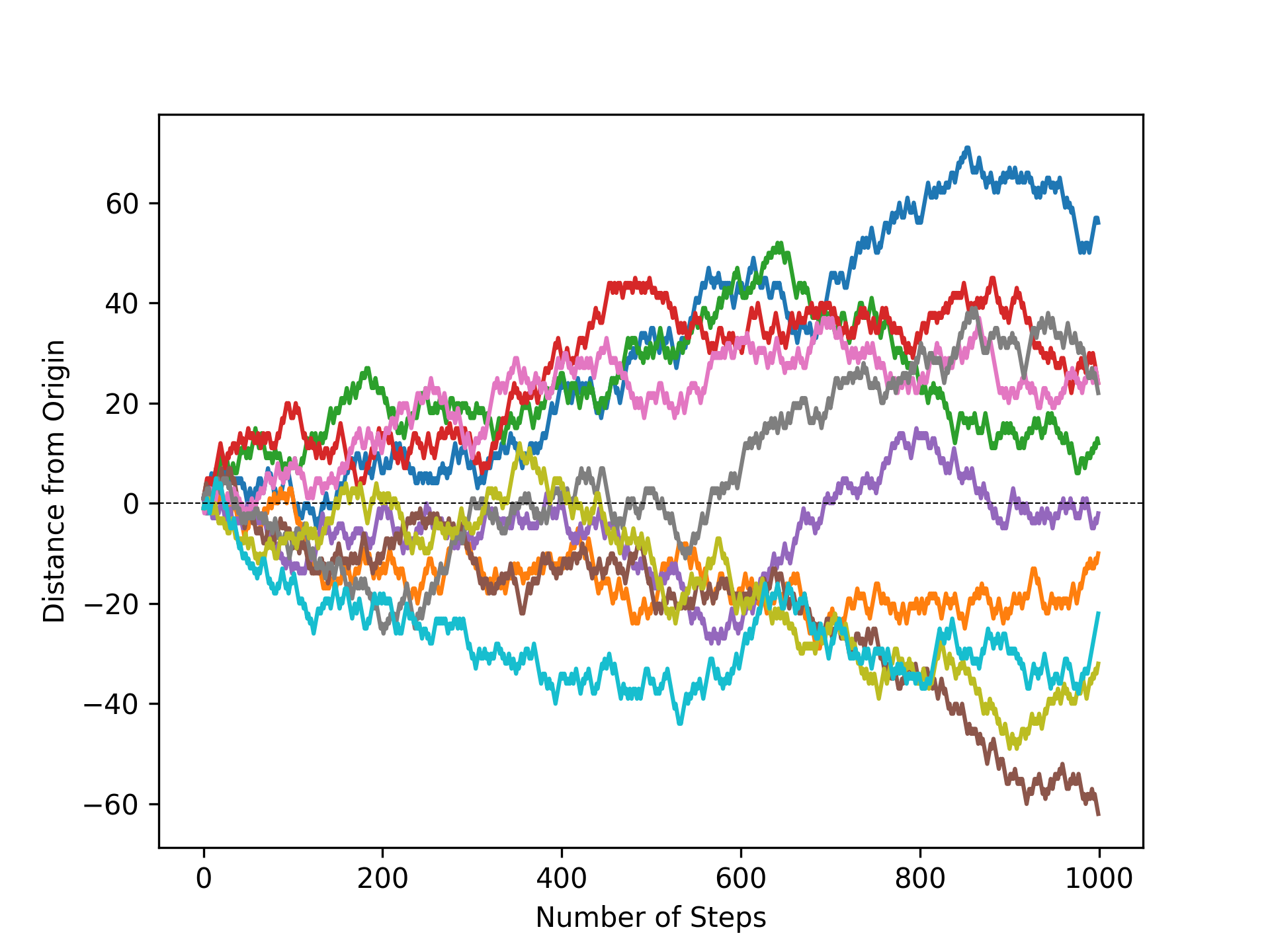
Fig. 63 Some random walk trajectories after 1000 steps.#
Quantum Random Walks - Introduction#
Firstly we need a way of encoding position into a set of qubits. If we have \(n\) qubits then each basis state can serve as a position by converting the binary string into an integer. E.g. the state \(|0110\rangle\) would be position 6, \(|6\rangle\).
For \(n=2\) the positions would be:
Basis State |
Position |
|---|---|
00 |
0 |
01 |
1 |
10 |
2 |
11 |
3 |
Consider two unitaries; one for a ‘step’ to the left and another for a ‘step’ to the right
Note that since \(U_LU_R=I\) the two are hermitian conjugates of each other: \(U_L=U_R^\dagger\), \(U_R=U_L^\dagger\) i.e. \(U_L\) undoes \(U_R\).
Thus for example in \(n=2\) case \(U_R |01\rangle = |10\rangle\), i.e. a step from position 1 to 2.
We have an issue though, what will happen when we apply \(U_L\) on the lowest position (\(0\))? Or \(U_R\) to the highest position (\(2^n-1\))?
I.e. in the \(n=2\) case what is
To ensure the operators are unitary we need the positions to be on a circle, i.e.

Fig. 64 The \(U_L\) and \(U_R\) operators on a circle.#
We want to find a unitary that does a ‘walk’ similar to the classical random walk.
Here’s one way to implement a quantum walk. We need a circuit composed of two registers \(|x,y\rangle\) where
The first register comprises a single qubit.
The second register encodes position (as before).
Consider the unitary \(U\) where
i.e. if the qubit in the first register is 0 (1) we step to the left (right).
By itself, this unitary doesn’t do anything very interesting. For example if we start in the state \(|0,j\rangle\) then applying \(U\) \(k\) times results in state \(|0,j-k\rangle\).
Instead, we combine with unitary with a Hadamard gate on the first register: \(U(H\otimes I)\)
i.e. \(50\%\) in position \(j-1\) and \(50\%\) in \(j+1\). This looks like a random walk!
Quantum Random Walks - Circuit#
The Quantum random walk algorithm is
Prepare an initial state, e.g. \(|0,j\rangle\)
Apply \(U(H\otimes I)\) for a given number of steps
Measure the second register
Find the position by converting the measurement to an integer
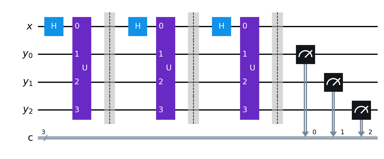
Fig. 65 The circuit for Quantum random walks.#
This looks very similar to Grover’s algorithm!
Quantum Random Walks - Results#
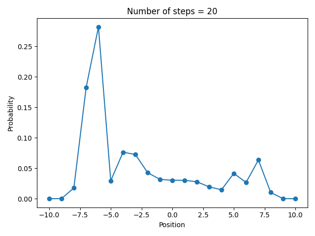
Fig. 66 Results for initial state: \(|0,0\rangle\)#
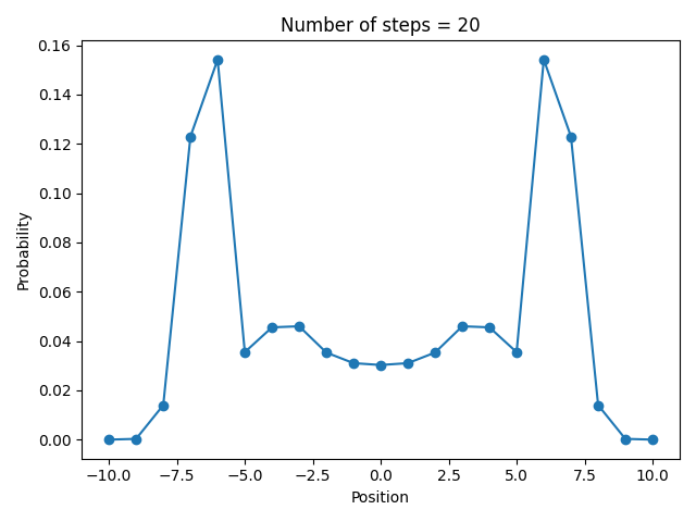
Fig. 67 Results for initial state: \(\frac{1}{\sqrt 2}(|0,0\rangle+i|1,0\rangle)\)#
Thus we see important differences between classical and quantum random walks (recall \(n\) is the number of steps):
Classical |
Quantum |
|
|---|---|---|
Distribution Symmetric |
Always |
Sometimes |
Distribution Shape |
Gaussian |
Non-Gaussian |
Variance (\(\sigma^2\)) |
\(n\) |
\(\propto n^2\) |
The fact that the variance of the Quantum distibution is \(n^2\) means the Quantum walks are ‘faster’ than the classical
The \(n^2\) variance can be seen by the fact that there are peaks far from the origin.
The differences between the classical and quantum cases are caused by interference.
Thus we see that for this simple classical algorithm the quantum version displays very different phenomena.
Use cases of quantum random walks include:
Finding marked items on a graph faster than classical search (similar to Grover’s algorithm but adapted to spatial structures like grids).
Evaluating whether a set of elements are distinct faster than classical algorithms.