Lecture 10: Early Quantum Algorithms

Lecture 10: Early Quantum Algorithms#

Warning

These lecture notes are a work in progress and are not a replacement for watching the lecture video, it’s intended to be a supplementary reading after watching the lecture

Learning Outcomes

In this learning we will continue with our exporation of early quantum algorithms. Specially we’ll discuss:

Simon’s Algorithm.
Shor’s Algorithm.
Grover’s Algorithm.

Simon’s Algorithm#

Simon’s algorithm was the first proposed quantum algorithm to demonstrate an exponential speed up over classical computers. While it doesn’t have a known practical use, it served as an inspiration for many other quantum algorithms.

Simon’s Problem#

Let \(f:\{0, 1\}^n \rightarrow \{0,1\}^n\) be a function that is 2-1 (for every \(x\) there is a \(y\) such that \(f(x)=f(y)\)) and where \(f(x\,\text{XOR}\, c)=f(x)\). Our task is to find \(c\).

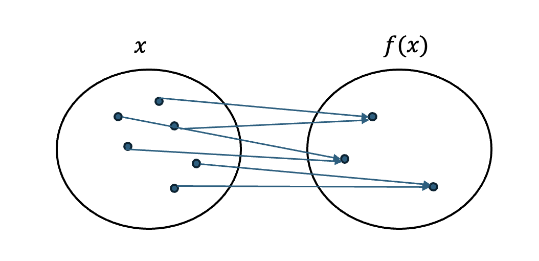
../_images/two-one-func.png — Fig. 28 A 2-1 function, here for every output there are two inputs that map to it.#

Here \(x\,\text{XOR}\, c\) means to take the component-wise XOR between the n-bit strings \(x\) and \(c\). If \(x=1011\) and \(c=0101\) then we would get \(x\,\text{XOR}\, c=1110\).

Classically this can be solved with an average of \(O(2^{n/2})\) evaluations. While on a quantum computer on average we will require only \(O(n)\) evaluations.

Quantum Speed up#

With \(2n\) qubits split into 2 n-bit registers, Simon’s algorithm consists in the following steps:

Firstly we apply a Hadamard gate to each qubit in the first register, creating the state

\[ \frac{1}{2^{n/2}} \sum_x |x\rangle |0\rangle. \]

Note that the sum is over all n-bit strings, so for \(n=2\) we sum over \(00\), \(01\), \(10\) and \(11\).

Then we apply the unitary \(U|x\rangle|y\rangle=|x\rangle|y \,\text{XOR}\, f(x) \rangle\) getting the state

\[ \frac{1}{2^{n/2}} \sum_x |x\rangle |f(x)\rangle. \]

Next we measure the qubits in the second register. Suppose we measured \(f(z)\), where recall \(f(z)\) is an n-bit string, then we know that qubits in the first register must either be in \(z\) or \(z \,\text{XOR}\, c\) and hence the qubits in the first register are in state

\[ \frac{|z\rangle + |z \,\text{XOR}\, c\rangle}{\sqrt 2} \]

Now we apply a Hadamard gate again to each qubit in the first register producing the state

\[\begin{split} \frac{1}{2^{(n+1)/2}} \sum_x [(-1)^{x\cdot z} + (-1)^{x\cdot (z \,\text{XOR}\, c)}|x\rangle \\ \end{split}\]

where \(x\cdot z=x_1 z_1 + x_2 z_2 + ... + x_n z_n\). Using the fact that \((-1)^{a \,\text{XOR}\, b}=(-1)^{a+b}\) where \(a,b\in\{0,1\}\) we can rewrite this as

\[\begin{split} \begin{split} & \frac{1}{2^{(n+1)/2}} \sum_x [(-1)^{x\cdot z} + (-1)^{x\cdot z} (-1)^{x\cdot c}|x\rangle \\ =& \frac{1}{2^{(n+1)/2}} \sum_x (-1)^{x\cdot z}[1 + (-1)^{x\cdot c}|x\rangle .\\ \end{split} \end{split}\]

When \(x\cdot c\) is an odd number \(1 + (-1)^{x\cdot c}\) will be zero, thus we can simplify this as

\[ \frac{1}{2^{(n+1)/2}} \sum_{x|x\cdot c \in\, \text{even}} (-1)^{x\cdot z} |x\rangle \]

where \(x\cdot c \in\, \text{even}\) means we only sum over bit strings for which \(x\cdot c\) is an even number.

Thus running the above circuit once, the first register gives us a value of \(x\) for which \(x\cdot c\) is even. If we repeat this \(n\) times we will end up with \(n\) independent equations (assuming we don’t get duplicate values of \(x\)) for which we can easily solve for \(c\).

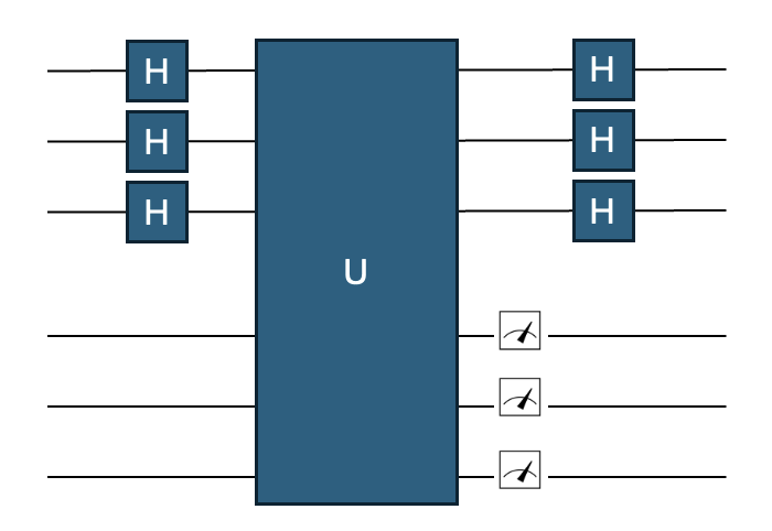
../_images/simons_circuit.png — Fig. 29 The circuit for Simon’s algorithm for \(n=3\).#

Shor’s Algorithm#

The fundamental theorem of arithmetic states that every integer can be unique written as a product of primes. For example the number \(42\) can be written as \(2*3*7\), all of which are prime. Shor’s algorithm can find the prime factors of a given integer exponentially faster than the best known classical algorithms.

Overview#

Shor’s algorithm consists of two steps:

Reduce the factoring problem to an order finding problem
Efficiently solve the order finding problem using the QPE algorihm

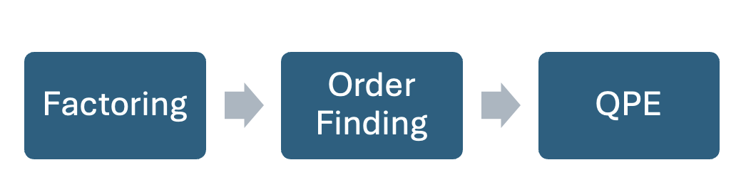
../_images/shor_workflow.png — Fig. 30 The workflow for Shor’s algorithm.#

The order finding problem is to find a value of \(r\) such that

\[ x^r = 1\, \text{mod}\, N \]

where \(0<x<N\). Here \(\text{mod}\, N\) means we divide by \(N\) and keep the remainder. It turns out that if we have a fast method for order finding, then we also have a fast method for factoring numbers.

Order finding can be efficiently run on a quantum computer using the QPE algorithm with unitary

\[ U|y\rangle=|xy\,\text{mod}\,N\rangle. \]

Implications for crytography#

In public-key cryptography one party is able to to securely share information to another, by using a public key (available to anyone) to encrypt a message and a private key (kept private by the party receiving the message) to decryt the message.

A common way to generate the public and private keys is to use the RSA algorithm. Here the protocal is as follows:

Choose two random prime numbers \(p\) and \(q\)
Compute \(n=pq\)
Compute \(\phi=(p-1)(q-1)\)
Select a random number \(e\) whose greatest common factor with \(\phi\) is 1
Find \(d\) where \(de=1\,\text{mod}\,\phi\)

The public keys are \((e, n)\) and the private key is \(d\). A message \(m\) can be encrypted using

\[ E(m) = m^e \,\text{mod}\, n \]

and decrypted using

\[ m = E(m)^d \,\text{mod}\, n. \]

The security of RSA relies on the assumption that factoring is difficult and can’t be done efficiently, as far as we know this is true on classical computers, but Shor’s algorithm shows it’s not the case for quanutm computers. Currently quantum computers are not large enough to run Shor’s algorithm, but post quantum cryptography protocals are already being adopted.

Grover’s Algorithm#

Grover’s algorithm is an algorithm for searching through an unstructed database. It ofters a quadratic speed-up over classical approaches.

Unstructured search#

We can formulate the search problem more formally as follows: Suppose we’re given a function

\[ f:\{0,1\}^n \rightarrow \{0,1\} \]

Our goal is to find a solution, which is a binary string \(x\in\{0,1\}^n\) for which \(f(x)=1\).

Classically we can solve this by iterating through all \(x\) and evaluating \(f\) on each one and stopping when we find \(f(x)=1\). If there are \(N\) elements in the list and only one solution then on average we will have to evaluate \(N/2\) elements.

Circuit#

For a database of size \(N=2^n\) we require \(n\) qubits. We define the oracle, \(O\), which performs the operation

\[ O|x\rangle = (-1)^{f(x)}|x\rangle. \]

We also define the Diffusion operator which performs the operation

\[ 2|\psi\rangle\langle \psi|-I \]

where \(|\psi\rangle\) is the uniform superposition state given by

\[ |\psi\rangle = \frac{1}{2^{n/2}} \sum_x |x\rangle \]

(note that the sum is over all \(n\) bit strings \(x\)) and \(I\) is the identity matrix.

Grover’s operator, \(G\), is defined as

\[ G = (2|\psi\rangle\langle \psi|-I)O \]

Grover’s algorithm consists in

Apply a Hadamard gate to each qubit (creating a uniform superposition state)
Apply Grover’s operator \(\sim\sqrt{N}\) times
Meaure the qubits

with a probability of at least \(1/2\) a solution will be measured.

WHy does Grover’s algorithm work?#

We define \(M\) to be the number of solutions (i.e. values of \(x\) for which \(f(x)=1\)).

We define an equal superposition of solutions

\[ |A_1\rangle = \frac{1}{\sqrt M} \sum_{x \,|\, f(x)=1}|x\rangle \]

where we some over all bit strings \(x\) which have \(f(x)=1\), and an equal superposition of non-solutions

\[ |A_0\rangle = \frac{1}{\sqrt{N-M}} \sum_{x \,|\, f(x)=0}|x\rangle. \]

Note that we can write the uniform superposition state \(|\psi\rangle\) in terms of these two states

\[\begin{split} \begin{split} |\psi\rangle &= \frac{1}{\sqrt N} \sum_x |x\rangle \\ &= \frac{1}{\sqrt N} \sum_{x \,|\, f(x)=0} |x\rangle + \frac{1}{\sqrt N} \sum_{x \,|\, f(x)=1} |x\rangle \\ &= \sqrt{\frac{N-M}{N}} |A_0\rangle + \sqrt{\frac{M}{N}} |A_1\rangle \\ &= \sqrt{1-\phi} |A_0\rangle + \sqrt{\phi} |A_1\rangle \\ \end{split} \end{split}\]

where we have defined \(\phi=M / N\).

Consider a linear combination of \(|A_0\rangle\) and \(|A_1\rangle\)

\[ |\alpha\rangle = a_0 |A_0\rangle + a_1 |A_1\rangle \]

note that the state the circuit is in before the first application of Grover’s application is \(|\psi\rangle\) and hence is in the form of \(|\alpha\rangle\).

If we apply Grover’s operator to \(|\alpha\rangle\) we get

\[\begin{split} \begin{split} G|\alpha\rangle &= (2|\psi\rangle\langle \psi|-I)O (a_0 |A_0\rangle + a_1 |A_1\rangle) \\ &= (2|\psi\rangle\langle \psi|-I)(a_0 |A_0\rangle - a_1 |A_1\rangle) \\ &= 2a_0 |\psi\rangle\langle \psi|A_0\rangle - 2 a_1 |\psi\rangle\langle \psi|A_1\rangle - a_0 |A_0\rangle + a_1 |A_1\rangle \\ &= 2a_0 \sqrt{1-\phi} |\psi\rangle - 2 a_1 \sqrt{\phi} |\psi\rangle - a_0 |A_0\rangle + a_1 |A_1\rangle \\ &= \left[a_0(1-2\phi) - 2 a_1 \sqrt{\phi(1-\phi)} \right] |A_0\rangle + \left[a_1(1- 2\phi) + 2a_0 \sqrt{\phi(1-\phi)} \right] |A_1\rangle .\\ \end{split} \end{split}\]

Note that \(0 \le \phi \le 1\) and hence \(-1 \le 1-2\phi \le 1\), this means we can write

\[ 1-2\phi = \cos \theta \]

and hence

\[ \sin \theta = \sqrt{1 - \cos^2 \theta} = \sqrt{1 - (1-2\phi )^2} = 2\sqrt{\phi(1-\phi)}. \]

Thus using this new \(\theta\) variable we get

\[\begin{split} G|\alpha\rangle = \left[a_0\cos \theta - 2 a_1 \sin \theta \right] |A_0\rangle + \left[a_1\cos \theta + 2a_0 \sin \theta \right] |A_1\rangle .\\ \end{split}\]

In terms of the coefficients \(a_0\) and \(a_1\), applying Grover’s operator to \(|\alpha\rangle\) results in the transformation

\[\begin{split} \begin{pmatrix} a_0\\ a_1\\ \end{pmatrix} \rightarrow \begin{pmatrix} \cos\theta & -\sin\theta \\ \sin\theta & \cos\theta \\ \end{pmatrix} \begin{pmatrix} a_0\\ a_1\\ \end{pmatrix}. \end{split}\]

In the 2-D plane with \(|A_0\rangle\) being the x-axis and \(|A_1\rangle\) being the y-axis, this corresponds to an anti-clockwise rotation of angle \(\theta\).

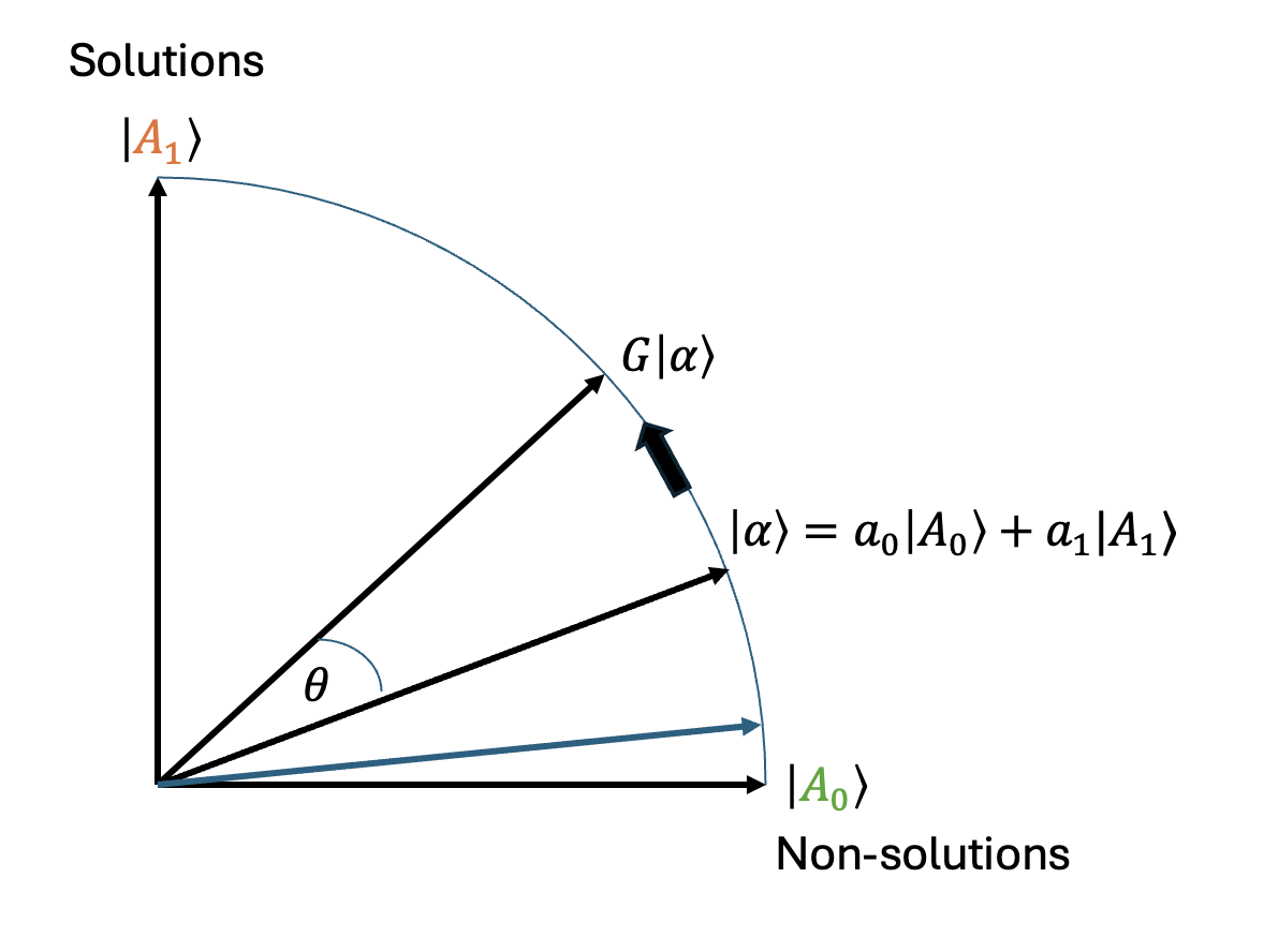
../_images/grover_rotation.png — Fig. 31 Applying Grover’s operator to state \(|\alpha\rangle\) results in an anti-clockwise rotation.#

Let’s suppose that the number of solutions \(M\) is small, then \(\phi=M/N\) must also be small. Thus we can approximate \(\phi(1-\phi)\approx \phi\) and hence \(\sin \theta = 2\sqrt{\phi(1-\phi)} \approx 2\sqrt{\phi}\). But if \(\phi\) is small then we can approximate \(\sin \theta\approx \theta\) and hence we end up with

\[ \theta \approx 2\sqrt{\phi} = 2\sqrt{\frac{M}{N}}. \]

Recall that the first step of Grover’s algorithm is to apply a Hadamard gate to each qubit, creating the uniform superposition state \(|\psi\rangle\), if \(M\) is small then \(|\psi\rangle\approx |A_0\rangle\). Thus we start very close to the \(|A_0\rangle\) state, recall that Grover’s operator rotates anticlockwise by angle \(\theta\), if we wish to end up near the \(|A_1\rangle\) we need to rotate by \(90\) degrees or \(\pi/2\) radians. Thus the number of rotations we require, \(k\), is

\[ k = \frac{\pi}{2 \theta} = \frac{\pi}{4} \sqrt{\frac{N}{M}}. \]

Thus we have derived the \(O(\sqrt N)\) scaling of Grover’s algorithm.

Limiations of early quantum algorithms#

Most early quantum algorithms require:

Large amounts of qubits
Long circuits
Error correction (to be robust in the present of noise), further increasing the number of required qubits

As current hardware is unable to meet these requirements, they are rarely used currently, with NISQ (Noisy Intermediate Scale Quantum) algorithms being developed and used instead.