Lecture 4: Mathematical framework for Quantum Computing

Warning

These lecture notes are a work in progress and are not a replacement for watching the lecture video, it’s intended to be a supplementary reading after watching the lecture

Learning outcomes

In this lecture we discuss the mathematical framework and tools required to properly understand how quantum system works. We give a short introduction to notion of vector spaces, linear operators, and how they connect to physical reality.

Postulates of Quantum Physics

Let us go through some of the building blocks of quantum mechanics, and see how the required mathematical framework emerges.

Uncertainty Principle

It is a fundamental principle of quantum mechanics, which states that certain pairs of physical properties can’t be measured simultaneously with arbitrary precision, for example a particle’s position and momentum. The properties which can form such pairs are called conjugate properties to each other. In the coming sections we will discuss more about them. In fact the product of uncertainties of the conjugate properties is bounded below. If the conjugate properties are \(A\) and \(B\), and the standard deviation or uncertainties in their simulaneous measurement in a given experiment are \(\sigma_A\) and \(\sigma_B\), then

\[ \sigma_A \sigma_B \ge \frac{h}{4\pi} \]

where \(h\) is Plank’s constant.

State as an abstract vector

In everyday life we use the term state when we refer to the situation/condition somebody or something is in. We make it more comprehensive by adding adjectives to it, such as in state of weakness, in state of pain, etc. In case of a physical system, the same idea extends to a comprehensive definition, with quantifiability. The state of a physical system refers to something that can provide complete physically accessible information about the system at a given instant of time. This is quantified with first determining the number of independent quantities required for complete information, and then assigning a variable for each of those. A numerical value of each of those variable defines the state of the system. Formally -

A state is a set of variables describing a system which does not include anything about its history.

This set of variable is assumed to be minimal so that removing any component results in only partial information about the system. Take for example the case of a single isolated particle. Then it’s position and velocity are two independent minimal properties. If the motion of this particle is constrained along a line, then a variable \(x\) denoting it’s distance from a chosen origin on the line completely determines it’s position, and it’s time derivative \(v = \frac{dx}{dt}\) determines the velocity. Thus together, \((x, v)\) define the state of the particle. If the motion was not constrained, one would need three coordinates \((x, y, z)\) for position, and three components of velocity \((v_x, v_y, v_z)\) with respect to a given reference frame. Thus collectively a set of six variables \((x, y, z, v_x, v_y, v_z)\) defines the state of a particle. For a system of many particles, the variables are concatenated, and the set becomes bigger. For \(N\) particle system, the set contains \(6N\) variables.

Note that this set has to be ordered so there is no confusion in the meaning of each of its elements. Such ordered sets are essentially what one calls vectors. We discuss vectors in more details in the coming sections.

Add Figure

A reference frame refers to a chosen point of origin, and a given orientation of coordinate axes in which a position is measured.

Degrees of Freedom

The degrees of freedom of a system is a number associated with it. It is the number of independent ways one can change the system’s state. Alternatively, it’s also the minimum number of individual quantities required to specify the state.

In case of single particle, it’s degrees of freedom is 6. For a system of \(N\) particles, it’s \(6N\).

Now consider a quantum particle, and think whether we can use the above mentioned set of positions and velocities/momenta \((x, y, z, v_x, v_y, v_z)\) can describe the state of quantum particle. Due to uncertainty principle, we immediately run into a problem, because the position \(x\), and velocity \(v_x\) can not be accurately determined simultaneously. Thus the set of position and velocity variables can not provide complete information about particle’s state.

So how do we define state of a quantum system? Here one postulates, that it is possible to define a state of a quantum system, represented as some type of abstract object. This object will likely have multiple components associated with it, one for each degree of freedom. It will thus be a vector of some kind. For the moment we call it an abstract vector, as we don’t know it’s structure. As we go throught the sections, we will explore how this structure emerges, and how it works.

So, for the moment, we say that the state of a quantum system is represented by an abstract vector. In due course we will learn several synonyms for this abstract vector defining the state of a quantum system.

---

Superposition principle

Superposition, issentially means applying multiple effect/stimuli/attributes on a system/object.

In general, the superposition principle applies to anywhere more than one attributes can be imposed on a single object. Formally speaking, the principle states that in all linear systems, the net response caused by two or more stimuli on a system is sum of the individual responses that would have been caused by each individual stimulus.

The sum of responses of individual effects, is same as the response of the sum of individual effecs.

Once we go through the mathematical structure in the coming sections, it will become clear that the superposition principle issentially is a consequence of linearity in the system, or linear behaviour.

In quantum mechanics, the superposition applies to states. What that means is, that if a system can exist in say two states \(A\) and \(B\), then it can also exist in a superposition of \(A\) and \(B\). In the section below we will learn how to interpret such a thing mathematically, but for now we can intuitively speculate, that a superposition of two states should have properties resembling both the states even though the two state might be very different.

Figure for illustration

Role of interference

The notion of intereference is quantum systems is very similar to what it means in waves. When two waves are combined, their instantaneous intensities or displacements are added. The intensity or displacement of the resulting wave can be greater or lower depending on their relative phase.

In case of quantum system, as we will see, probability amplitudes take the role of intensity or displacements.

Principles of measurement

In quantum mechanics, a measurement is testing or manipulation of a physical system that yields a numerical result. This in principle doesn’t look much different than a measurement of a classical system. However, in the quantum realm, the process of measureing something also changes the underlying system.

No-cloning

Entanglement

Tunnelling

---

Mathematica Structure

Here we discuss in bravety the necessary mathematical structures upon which the formulation of quantum mechanics relies on. It progressively goes as follows -

        mindmap
root(Mathematical Framework)
    Vector Space, Hilbert Space
        Scalar vs Vector
        States as Vector (Bra and Ket)
    Linear combination
        Linear independence
    Inner Product
        Overlap of vectors
        Orthogonality
    Linear Operators
        Commutativity
        Special operators: Unitary, Hermitian, ...
        Probability conservation
    Representation theory
    

Scalar vs Vector

Any quantity that can be described by a single numerical value, usually with real, and sometimes with complex numbers is a scalar. The common examples of scalars are volume, density, speed, energy, mass and time.

Quantities require multiples of numerical values, with each value describing some aspect or attribute of the quantities, are called vectors. The number of these values is called the dimension of the vector. Common examples of vector quantities from physics include position, velocity, momentum, and force. They all have two common attributes, (i) a magnitude, and (ii) a direction associated with them.

Both scalars and vectors are represented usually with real numbers, and often with complex numbers. So the notions of addition, subtraction, multiplication and division, through which we manipulate numbers, are suitably extended on scalars and vectors.

Scalars: are expressed in terms of single number, so their algebra is essentially the same as algebra of real/complex numbers they are expressed in.

Vectors: are expressed in terms of multiple numbers. So it’s not straight forward as to how to manipulate vectors, based on scalars, or formally extend their algebra from the component numbers. We see below how this is done.

Vector Space, Hilbert Space: A Vector space is a mathematical structure, that constitutes the necessary components to manipulate vectors in sensible way. Before we define it, we need to understand a few definitions, namely Set, map, Binary operations, Group and Field -

Set

Learning the notion of sets, and their manipulation provide not only training in fundamentals of logic of categorisation, organisation, it is crucial building block of most of mathematics.

In Mathematics, a set is defined as a unique collection of well defined objects[1], and the object in the collection are called elements of the set.

For example,

• \(A=\{a, e, i, o, u\}\) is a set of vowels in english language.

• \(\mathbb{Z} = \{0, \pm1, \pm2, \pm3,\dots\}\) is the set of integers.

It’s important to imphesise the important of uniqueness in a set. It means in that in a set, a member exists only once. Thus \(A=\{a, e, i, o, u\}\) is a well defined set, while \(A=\{a, e, i, o, u, a, i\}\) is not, as \(a, i\) are put twice. So a set is different than a mere list, which can have multiple occurrance of an object.

Secondly, the order of elements in a set have no meaning, so \(\{a, e, i, o, u\}\) and say, \(\{i, o, a, u, e\}\) are same sets, just expressed differently.

A set is expressed with mainly two ways:

1. Roster method: This is the method where we list all the elements of the set, in no particular order, and put them in curly braces. The set of vowels, \(\{a, e, i, o, u\}\) is one such examples. It is the simplest method, but becomes inconvenient for sets with large number of elements, or infinite number of elements.

2. Set builder/logical method: In this method, instead of trying to list elements one by one, we name a representative element, and describe it’s specific properties that make it a member of the set. For example, see below, and example of set builder method.

\[ B = \{a| a\in \mathbb{Z}, \text{ and } a \text{ is even}\} \]

The above is seen or read as “B equals a set of all ‘\(a\)’ such that \(a\) is an integer, and \(a\) is even”. Equivalently, B is set of all even integers. The roster version of this would be \(B = \{\dots, -3, -2, -1, 0, 1, 2, 3, \dots\}\).

A set can be finite, or infinite, that is, the number of elements in a set can be finite, or infinite.

You can manipulate a set, by adding or removing elements from it. A set with no elements is called Null set, denoted by \(\emptyset\).

Sets can be finite and infinite. We all know what being finite is, so a finite set is a set with finite number of elements which one could count.

Infinite is a slightly tricky concept in mathematics. To start with, an infinite set is a set that is not finite.

The set of natural numbers \(\mathbb{N} = \{1, 2, 3, \dots\}\) plays a central role in the categorisation of sets. First, it let’s us define countability. So a set in which you could count the number of elements one by one, is called countable. If the counting finishes after finite number, the set is finite and countable. If you can count, and the counting can not finish in finite time, the set is said to be countably infinite. By definition or axiom, the set of natural number is countably infinite. Uncountable sets on the other hand, are the ones that are inifinite, and contains too many elements to be even countable.

We use the term cardinality for representing a measure of number of elements in a set. The cardinality of a finite set is the number of elements in it. For infinite sets, the cardinality is symbolic and is established by comparison of two sets and defining map among them.

Subsets

Imagine we have two sets, A and B, and it is such that, every element of A is also element of B, then we say that A is a subset of B. It is denoted as \(A\subset B\). We also in this case, call B as superset of A.

Naturally, every set is subset and superset of itself. We a call a set A to be a proper subset of B, if every element of A is in B, but at least one element exists in B that is not in A. In this case, B is called a proper superset of A.

For finite sets, their proper subsets have strictly lower number of element than the set itself. However for infinite sets, a proper subset may have same cardinality as the set itself.

Fig. 4 A is subset of B, and B is superset of A

Fig. 5 Visualisation of the set of numbers, natural numbers \(\mathbb{N}\), integers \(\mathbb{Z}\), rational numbers \(\mathbb{Q}\), real numbers \(\mathbb{R}\), and complex numbers \(\mathbb{C}\). We have following \(\mathbb{N}\subset \mathbb{Z}\subset \mathbb{Q}\subset \mathbb{R}\subset \mathbb{C}\)

We defined what a set is, and introduced a notion of comparison by defining what a subset, and superset is. There is a lot more one can do with the notion of sets, to manipulate them, to the extent that it looks like everyday algebra.

• Universal set: For a given consideration of problem, a universal set \(U\) is set of all elements considered, and fixed, so that every set defined for the problem, is a subset of \(U\).

• Complement: Compliment of a set A, denoted by \(A'\), or sometimes \(A^c\) is defined with respect to the universal set, is set of all elements of \(U\) that are not in A.

Fig. 6 Set Union, intersection and set difference.

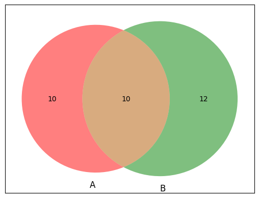
• Union: A union of two sets, say A and B, denoted as \(A\cup B\) is defined as the set of all elements that belong to either A, or B, or both. For example, if \(A=\{1,2,3,4\}\) and \(B=\{1,3,5,7\}\), then

\[A\cup B = \{1, 2, 3, 4, 5, 7\}\]

• Intersection: An intersection of two sets, say A and B, denoted as \(A\cap B\) is defined as set of all elements that belong to both A and B.

• Difference: The set difference of A from B, denote as \(A-B\), is set of all elements of A that are not elements of B.

• Cartesian Product: A cartesian product of two sets, say A and B, denoted by \(A\times B\) is the set of all ordered pairs \((a, b)\) such that \(a\) belongs to A, and \(b\) belongs to B.

For examples, if \(A=\{a, b, c\}\) and \(B=\{x, y, z\}\) then

\[ A\times B = \{(a, x), (a, y), (a, z), (b, x), (b, y), (b, z), (c, x), (c, y), (c, z)\} \]

Map

In mathematics, a map is somethings that defines a symbolic relation from elements of a set X to elements of another set Y, such that each element of X gets associated to an element of Y. The set X whose elemets get mapped to is called the domain of the map and the set Y the elements of which they get mapped from is called the range or codomain of the map.

Symbolically, a map is expressed as follows

• We say that \(f\) is a map from X to Y by \(f: X\longrightarrow Y\)

• For an element \(x\) in X, the element in Y it maps to, is expressed as \(f(x)\).

• The element \(f(x)\) belongs to Y, and is called the image of \(x\).

• The map, mapping, correspondence are synonyms. Usually, if the set is of numbers, they are also called functions.

• A map between two sets let’s us see a holistic relation between them.

• If distinct elements of the domain set X get mapped to distinct elements of the codomain set Y, the map is called injective, or one-to-one. For example, consider the set of integers \(\mathbb{Z}\), and a map \(f: \mathbb{Z} \longrightarrow \mathbb{Z} \) such that \(f(x) = 3 x\). This is an injective map from \(\mathbb{Z}\) to itself.

• A map in which each element of the codomain set is image of some element in domain set, is called surjective or on-to map.

• A map that is both injective, and surjective, is called a bijective map. Bijective maps play an important role in mathematics.

• Recall the uncountable sets. Using concept of map we can more clearly define it as follows - A set X is uncountable if and only if there exists no injective map from the set X to set of natural numbers \(\mathbb{N}\).

• Consider the set of integers \(\mathbb{Z}=\{\dots, -2, -1, 0, 1, 2, \dots\}\) and a map \(f:\mathbb{Z}\longrightarrow \mathbb{Z};\quad f(n)=3n\). The range of this set is a proper subset of \(\mathbb{Z}\), as the range only contains numbers that are multiple of 3. However, since the map is injective, this means that the subset has the same cardinality as \(\mathbb{Z}\).

\[\begin{split} \begin{align} \begin{Bmatrix} \vdots \\ -2\\ -1\\ 0\\ 1\\ 2\\ \vdots \end{Bmatrix} \underrightarrow{~~~~~~f~~~~~~} \begin{Bmatrix} \vdots \\ -6\\ -3\\ 0\\ 3\\ 6\\ \vdots \end{Bmatrix} \end{align} \end{split}\]

• Maps can be combined. Instead of exploring general consequences, consider two bijective maps \(f, g\) from a set X to itself. If \(f\) maps an arbitrary element \(a\) in X to \(b=f(a)\), and \(g\) maps \(b\) to \(c=g(b)\), then the the combination, or composition of the two maps \(fog\) maps \(a\) to \(fog(a) = f(g(a))\).

        graph LR
a(["X"])
b(["X"])
c(["X"])
a --f--> b --g--> c
a --fog--> c
    

Binary operations

Binary operations, as the name suggests are operations that take two objects and combine them to give (usually) one unique object.

In mathematics, binary operation is defined on a set, that takes two elements of the set, and returns one element of a set.

Formally, a binary operation on a set A is a mapping of elements of \(A\times A\) to A, expressed as

\[ o : A\times A \longrightarrow A \]

For the binary operation to be well defined, the operation \(o\) should be such that every pair of elements from A, should map to a unique element in A. That is, if \(a, b\) are two arbitrary elements of A, then there exists a \(c\) in A, that \(o(a, b) = c\). \(o(a, b)\) or \(a~o~b\) is denoted as result of the binary operation.

Commutativity A binary operation is said to be commutative, if the result of combining does not depend on which is combined to the other i.e., if \(a o b = b o a\) for every \(a, b\) in the set A.

Examples:

• On the set of real numbers \(\mathbb{R}\), the usual addition \(o(a,b) = a + b\), and the usual multiplication \(o(a,b) = ab\) are most common examples of binary operations.

• Consider a given set X, and a set S of all possible bijective maps from X to X, then the composition of maps o is a binary operation.

Group

When we have a set, it let’s us categorize, and organize the elements. Having binary operations defined on a set tells us how a pair of elements of the set result in another element, in effect how combining elements gives us different elements.

The binary operations defined on a set, give new structure to the set. A group is one such structure.

A group is a set \(A\) with an operation \(o\), expressed as \((A, o)\), such that the operation satifies following conditions -

1. Associativity A binary operation is called associative, if \(a o (b o c) = (a o b) o c\) for every elements \(a, b, c\) in \(A\).

2. Existence of Identity There exist an element \(e\) in \(A\) such that for every element \(a\in A\), \(e o a = a\), i.e., combining any element with \(e\) results in the same element.

3. Existence of Inverse For every element \(a\in A\), there exists another element, say \(a'\) such that \(a' o a = e\), i.e, combining the two results in indentity element.

The inverse of an element \(a\) is often denoted by \(a^{-1}\). There are certain consequence, that result directly out of the above three assumptions. Consider the identity in the group \((A, o)\): we said for identity, \(e o a = a\), and why not \(a o e = a\)?

The two expressions are in general different, and can potentially, mean existence of two types of identity elements, say left identity and right identity. However one can prove based on the purely logic, and the knowledge that \((A, o)\) is a group, that the left and right identities, are the same element.

The same question can be posed for the existence of the inverse. The left and the right inverses of an element (can be proven) are the same.

The inverse of the inverse of the element \(a\), is the element itself, i.e., \((a^{-1})^{-1} = a\)

Subgroups

Just like sets have subsets, groups have subgroups. A subgroup of a group \((G, o)\) is a subset \(S\subset G\), that forms group under the binary operation \(o\) of the group constrained within \(S\). So in order for a subset to be a subgroup, following must be satisfied

• The binary operation \(o\) defined on the set \(G\), is also a binary operation on the subset \(S\).

• The identity of \(o\), say \(e\) belongs to \(S\), and for every \(a\) in \(S\), \(a^{-1}\) also belongs to \(S\)

Examples

The set of integers with arithmatic addition \((\mathbb{Z}, +)\) forms a group.

The arithmatic operation + is a binary operation, as adding any two integers results in another, unique integer. Since the order of adding two integers, does not matter, the operation is obviously commutative.

Next, we know that addition of three numbers is associative (otherwise grocery shopping to stock markets, everything would have been a mess! 😀).

Zero is clearly the identity element in the set of integers.

For every number, it’s negative is the additive inverse.

• What about the set of rational numbers, real numbers and complex numbers. Do any of these form a group with arithmatic addition +, or multiplication * ? Following table gives a summary of answers, try to figure out why.

Set A	(A, +)	(A, .)	(\(A^*\), .)
\(\mathbb{Z}\)	Group	No	No
\(\mathbb{Q}\)	Group	No	Yes
\(\mathbb{R}\)	Group	No	Yes
\(\mathbb{C}\)	Group	No	Yes

Here \(A^* = A - {0}\), is the set with additive identity element removed from \(A\).

The above defines what a group is, and based on the above example it may look like that a group is just a formal abstract version of what we already know about numbers from our school algebra/arithmatic knowlege. However this abstraction leads to generalization of the arithmatic operation to sets of other objects. See the following examples -

Permutation Group

A permutation is an arrangement of elements of a set. As we know, a set does not have a notion order of elements. But if the order of the elements mattered, each permutation, seen as ordered sequence of elements, will look different, as in figure below.

Fig. 7 Each row represents an arrangement of the three balls of colour red, green and blue. There are 6 such arrangements.

To abstractify, instead of ball of three colours, consider a set of 3 objects, and without loss of generality we can call them \(a, b, c\). Now consider a set of each permutations of the three elements. The table below shows all possible arrangements of the three objects \(a, b, c\) symbolically represented as \(p_0, p_1, p_2...\).

	\(p_0\)	\(p_1\)	\(p_2\)	\(p_3\)	\(p_4\)	\(p_5\)
Sequence	(abc)	(acb)	(bac)	(bca)	(cab)	(cba)
Mapping	(123)	(132)	(213)	(231)	(312)	(321)

If we choose a reference arrangement to be \((a,b,c)\), then, \(p_0\) is a map that maps (abc) to it itself, \(p_1\) maps (abc) to (acb), and so on. Basically, \(p_0, p_1, ...\) are bijective maps which map (abc) to different arrangements. Below is a table that show how resulting maps of combining two maps.

They can be computed as following -

\[\begin{split} \begin{align} p_1 p_1(abc) &= p_1(acb) = (abc) = p_0(abc) \implies p_1p_1 = p_0\\ p_1 p_2(abc) &= p_1(bac) = (bac) = p_3(abc) \implies p_1p_2 = p_3\\ p_1 p_3(abc) &= p_1(bac) = (bac) = p_2(abc) \implies p_1p_3 = p_2\\ \dots &= \dots \end{align} \end{split}\]

Below is the operation table for composition \(o\). Row and column numbers correspond to first and second operand respectively (row \(o\) column).

\(o\)	\(p_0\)	\(p_1\)	\(p_2\)	\(p_3\)	\(p_4\)	\(p_5\)
\(p_0\)	\(\mathbf{p_0}\)	\(p_1\)	\(p_2\)	\(p_3\)	\(p_4\)	\(p_5\)
\(p_1\)	\(p_1\)	\(\mathbf{p_0}\)	\(p_3\)	\(p_2\)	\(p_5\)	\(p_4\)
\(p_2\)	\(p_2\)	\(p_4\)	\(\mathbf{p_0}\)	\(p_5\)	\(p_1\)	\(p_3\)
\(p_3\)	\(p_3\)	\(p_5\)	\(p_1\)	\(p_4\)	\(\mathbf{p_0}\)	\(p_2\)
\(p_4\)	\(p_4\)	\(p_2\)	\(p_5\)	\(\mathbf{p_0}\)	\(p_3\)	\(p_1\)
\(p_5\)	\(p_5\)	\(p_3\)	\(p_4\)	\(p_1\)	\(p_2\)	\(\mathbf{p_0}\)

If we consider the set \(P=\{p_0\, p_1, ..., p_5\}\), then the above composition \(o\) is a binary operation, and \((P, o)\) forms a group. Here \(p_0\), is the identity, as combining it with any other map gives the same map. Each element has an inverse, \(p_0, p_1, p_2, p_5\) are inverses of their own, and \(p_3\) and \(p_4\) are inverses of each other.

This is called permutation group. We showed the example of three objects, but the group generalises to any number of objects. For \(n\) object, the set of bijective maps has \(n!\) elements.

Group of modular arithmatic

Modular arithmatic is a system of arithmatic, where numbers wrap around after reaching a certain value. A common example is arithmatic of 12-hour clock. In general, consider a positive integer \(m > 1\). Now any arbitrary integer \(a\in \mathbb{Z}\), we can write \(a = qm + r\) where \(q, r\) are some integers. There is unique pair \(q, r\) such that \(q\) is largest, and \(0\le r\lt m\), in which case we know \(q\) and \(r\) as quotient and remainder when \(a\) is divided by \(m\). Since in this unique representation \(r\) can have only \(m\) possible values in set \(Z_m = \{0, 1, 2, \dots, m-1\}\).

On this set, we define modular addition \(\oplus\), to distinguish with usual addition + as follows:

For any two arbitrary \(a, b\) in \(Z_m\), \(a \oplus b = c\) where \(a + b = qm + c\), i.e, \(c\) is obtained by computing the remainder when \(a+b\) is divided by \(m\).

Then \((Z_m, \oplus)\) forms a group, because of following -

• \(\oplus\) is a binary operation, moreover, it is also commutative.

• 0 is the identity, for any \(a\oplus 0 = a\).

• For any \(a\) in \(Z_m\), \(0\le a\lt m\), there exists \(m-a\), such that \(a\oplus (m-a) = 0\), so \(m-a\) is the inverse of \(a\).

Illustration: Consider \((Z_{8}, \oplus)\), where \(Z_8 = \{0, 1, 2, 3, 4, 5, 6, 7\}\), then under modular arithmatic, \(2\oplus 3 = 5\), but \(4\oplus 4 = 0\) and \(4\oplus 7 = 3\)

Field

In mathematics, a field is defined as a set \(F\) with two binary operations, say + and . such that following conditions are satisfied -

1. The binary operations + and . are commutative, i.e., \(a + b = b + a\), and \(a\cdot b = b\cdot a\) for every \(a, b\in F\).

2. \((F, +)\) is a group. Let’s call 0 it’s identity for +.

3. \((F^*, \cdot)\) is also a group, where \(F^* = F - \{0\}\) is set with identity of + removed from it. Let’s call the identity for this as 1.

4. The operation . distributes over +, i.e., \(a\cdot (b + c) = (a\cdot b) + (a\cdot c)\) for every \(a, b, c \in F\).

Examples:

• The set of rational (\(\mathbb{Q}\)), real (\(\mathbb{R}\)), and complex numbers (\(\mathbb{C}\)), all from respective fields with usual arithmatic addition + and multiplication .. \((\mathbb{Q}, +, \cdot)\), \((\mathbb{R}, +, \cdot)\), \((\mathbb{C}, +, \cdot)\) are all fields, with 0 as additive identity, and 1 as multiplicative identity.

• There are examples of fields of finite set, but their discussion takes us (more than usual) different direction than we intend this lecture notes to. For most of the discussion, even the group aspect might be generally needed, the field of number relevant for us will be that of \((\mathbb{R}, +, \cdot)\) and \((\mathbb{C}, +, \cdot)\).

• Recall the modular arithmatic, where \((Z_m, \oplus)\) formed a group for any arbitrary positive integer \(m\). Now consider a modular version of the usual arithmatic multiplication, \(\odot\), defined as follows. If \(a, b\) are two arbitrary integers in \(Z_m\), then \(a\odot b = c\) where \(c\) is the remainder you get when you divide \(ab\) with \(m\). Does the \((Z_m, \oplus, \odot)\)

  • Clearly, \(\odot: Z_m\times Z_m \longrightarrow Z_m\) is a binary operation.

  • 1 is the multiplicative identity, as \(1 \odot a = a\) for every \(a\) in \(Z_m\).

  • However, unless \(m\) is prime, we have issues with the structure of identity and inverse.

  • Does every element has an inverse? Imagine \(a, b\) in \(Z_m\) are inverses of each other, then \(a\odot b = 1\), which means \(ab\) is of the form \(ab = qm + 1\), which means \(b= {qm + 1\over a}\)

Polynomials

We need the structure of a field, i.e., set with atleast two binary operations to construct expressions that we call polynomials.

Vector Space

All the above mathematical definitions, going through which can be perhaps excruciating, let us define what we need for the underlying math of quantum computing: A vector space, and a Hilbert space. We will see, that these two are nearly same structures, with one difference.

A vector space is a mathematical structure, that consists of two sets, which have the following substructures:

• The first set, say V, whose elements are called vectors, is a commutative group \((\mathbf{V}, +_v)\) with addition \(+_v\). Let’s call \(0_v\) the zero vector as the identity of this group.

• The second set, say F, whose elements are called scalars, is a Field \((F, +_f, \cdot_f)\) with addition \(+_f\) and multiplication \(\cdot_f\). Let’s call the \(0\) and \(1\) additive and multiplicative identity of the field.

• A binary operation \(\cdot : F\times V \longrightarrow V\) called scalar multiplication. This operation combines a scalar and a vector, and gives us a vector. It lets manipulate vectors through scalars, and satisfies following -

1. Associativity: For any arbitrary \(a, b\) in F, and any arbitrary \(\mathbf{v}\) in V,

\[a \cdot (b\cdot\mathbf{v}) = (a\cdot_f b)\mathbf{v}\]

This means multiplying a vector successively by two scalars gives the same vector, as when multiplying the field multiplication of those two scalars to the vector.

2. Distribution: The scalar multiplication distributes over addition of vectors, and addition of scalars. That is, for any arbitrary scalars \(a, b\) in F and any arbitrary vectors \(\mathbf{u, v}\) in V, the following holds

\[\begin{split} \begin{align*} a\cdot(\mathbf{u} +_v \mathbf{v}) &= (a\cdot\mathbf{u}) +_v (a\cdot\mathbf{v})\\ (a +_f b)\cdot \mathbf{v} &= (a\cdot\mathbf{v}) +_v (b\cdot\mathbf{v}) \end{align*} \end{split}\]

• Multiplying any scalar with zero vector gives zero vector, \(a\cdot 0_v = 0_v\), and multiplying zero scalar 0, with any vector gives zero vector, \(0\cdot v = 0_v\).

Because of associativity, and distribution of scalars with vectors, we often use the same symbol for addition (+ for \(+_v\) and \(+_f\)) and scalar multiplications (\(\cdot\) for \(\cdot_f\)).

Let us take a moment to appreciate what makes the structure of vector space rich. We have a set V of vectors elements, and set F of scalar elements. If one of the sets is infinite, the vector space automatically becomes infinite. (Guess Why?)

Examples:

Consider the set of points on 3D space, they are represented by the cartesian product of the set of real numbers

\[ \mathbb{R}^3 = \mathbb{R}\times \mathbb{R}\times \mathbb{R} = {(x, y, z): x, y, z\in \mathbb{R}} \]

If we define vector addition of two arbitrary points \(\mathbf{r_1}=(x_1, y_1, z_1)\), and \(\mathbf{r_2}=(x_2, y_2, z_2)\) as

\[ \mathbf{r_1} + \mathbf{r_2} = (x_1 + x_2, y_1 + y_2, z_1 + z_2) \]

then \(\mathbb{R}^3\) forms a vector space over the field of real numbers \((\mathbb{R}, +, \cdot)\).

Consider a toy example of ‘constructing a vector space’. Let there be a set of just two non-zero vectors \(\mathbf{V} = \{0, \mathbf{a_{\uparrow}}, \mathbf{a_{\downarrow}}\}\), where 0 is zero vector with respect to some addition operator ‘+’ which we define below. To define addition as binary operation, we have the following by definition of zero, or identity.

\[\begin{split} \mathbf{a_{\uparrow}} + 0 = 0 + \mathbf{a_{\uparrow}} = \mathbf{a_{\uparrow}}\\ \mathbf{a_{\downarrow}} + 0 = 0 + \mathbf{a_{\downarrow}} = \mathbf{a_{\downarrow}} \end{split}\]

But what about \(\mathbf{a_{\uparrow}} + \mathbf{a_{\downarrow}}\) ? It’s value can neither be \(\mathbf{a_{\uparrow}}\), nor \(\mathbf{a_{\downarrow}}\) as in either case, the other element becomes the identity, or 0.

\[ \text{If}\quad\mathbf{a_{\uparrow}} + \mathbf{a_{\downarrow}} = \mathbf{a_{\uparrow}} \implies \mathbf{a_{\downarrow}} = 0\quad\text{but we assumed it to be non-zero.} \]

Thus the only option within the set is \(\mathbf{a_{\uparrow}} + \mathbf{a_{\downarrow}} = 0\), which makes the two vectors inverse of each other. Now, what do we assign to \(\mathbf{a_{\uparrow}} + \mathbf{a_{\uparrow}}\), and \(\mathbf{a_{\downarrow}} + \mathbf{a_{\downarrow}}\)? We can’t have \(\mathbf{a_{\uparrow}} + \mathbf{a_{\uparrow}} = 0\) as this will make \(\mathbf{a_{\uparrow}} = 0\), and same argument holds for \(\mathbf{a_{\downarrow}}\). So the only option plaussible is \(\mathbf{a_{\uparrow}} + \mathbf{a_{\uparrow}} = \mathbf{a_{\downarrow}}\), and \(\mathbf{a_{\downarrow}} + \mathbf{a_{\downarrow}} = \mathbf{a_{\uparrow}}\).

This gives the structure of this three element group, where combining any non-zero element with itself gives the other element, and both non-zero elements are inverses of each other.

Other option, which gives us more to play with in context of vector space is, to assume that \(\mathbf{a_{\uparrow}} + \mathbf{a_{\downarrow}}\) should exist as separate vector in V. Moreover, if \(\mathbf{a_{\uparrow}}\) and \(\mathbf{a_{\downarrow}}\) aren’t inverses of each other like above, they should have separate inverses. This means that the set V should be extended to atleast

\[ \mathbf{V} \to \{0, \mathbf{a_{\uparrow}}, -\mathbf{a_{\uparrow}}, \mathbf{a_{\downarrow}}, -\mathbf{a_{\downarrow}}, \mathbf{a_{\uparrow}} + \mathbf{a_{\downarrow}}, -(\mathbf{a_{\uparrow}} + \mathbf{a_{\downarrow}})\} \]

With introduction of more elements, we have to again make sure that the binary operation is well defined, i.e., addition of any two element results an element in the set. Consider now the \(\mathbf{a_{\uparrow}} + (\mathbf{a_{\uparrow}} + \mathbf{a_{\downarrow}})\), just like previous exercise, its value can not be either of \(\mathbf{a_{\uparrow}}, \mathbf{a_{\downarrow}}\) or \(\mathbf{a_{\uparrow}} + \mathbf{a_{\downarrow}}\), otherwise either of these will result in a contradiction.

So, \(\mathbf{a_{\uparrow}} + (\mathbf{a_{\uparrow}} + \mathbf{a_{\downarrow}})\), and it’s inverse must now exist as seperate vector. We can simplify the expression \(\mathbf{a_{\uparrow}} + (\mathbf{a_{\uparrow}} + \mathbf{a_{\downarrow}})\) = \((\mathbf{a_{\uparrow}} + \mathbf{a_{\uparrow}}) + \mathbf{a_{\downarrow}}\) = \(2\mathbf{a_{\uparrow}} + \mathbf{a_{\downarrow}}\), where \(2\mathbf{a_{\uparrow}}\) symbolically means \(\mathbf{a_{\uparrow}} + \mathbf{a_{\uparrow}}\). We can easily see that

• This process of extending is actually endless

• If we keep doing this over and over again, the new elements added are expressed as some ‘combination’ of the originally assumed two non-zero vectors.

• We have deceptively used the notion of actual numbers to express new vectors.

• The fully extended set looks like

\[\begin{split} \mathbf{V} \to \{ 0, \mathbf{a_{\uparrow}}, -\mathbf{a_{\uparrow}}, \mathbf{a_{\downarrow}}, -\mathbf{a_{\downarrow}}, \mathbf{a_{\uparrow}} + \mathbf{a_{\downarrow}}, -(\mathbf{a_{\uparrow}} + \mathbf{a_{\downarrow}}), 2\mathbf{a_{\uparrow}} + \mathbf{a_{\downarrow}},-(2\mathbf{a_{\uparrow}} + \mathbf{a_{\downarrow}}),\\ \mathbf{a_{\uparrow}} + 2\mathbf{a_{\downarrow}},-(\mathbf{a_{\uparrow}} + 2\mathbf{a_{\downarrow}}), 3\mathbf{a_{\uparrow}} + \mathbf{a_{\downarrow}},-(3\mathbf{a_{\uparrow}} + \mathbf{a_{\downarrow}}), \mathbf{a_{\uparrow}} + 3\mathbf{a_{\downarrow}},-(\mathbf{a_{\uparrow}} + 3\mathbf{a_{\downarrow}}),\\ 2\mathbf{a_{\uparrow}} + 3\mathbf{a_{\downarrow}},-(2\mathbf{a_{\uparrow}} + 3\mathbf{a_{\downarrow}}), 3\mathbf{a_{\uparrow}} +2\mathbf{a_{\downarrow}},-(3\mathbf{a_{\uparrow}} + 2\mathbf{a_{\downarrow}}), \dots \} \end{split}\]

In a more compact form (albeit terse looking) the set looks like \(\mathbf{V} = \{n_1\mathbf{a_{\uparrow}} + n_2\mathbf{a_{\downarrow}}: \text{where}\quad n_1, n_2 \in \mathbb{Z}\}\), i.e., every element in the set is of the form \(n_1\mathbf{a_{\uparrow}} + n_2\mathbf{a_{\downarrow}}\) for some integers \(n_1, n_2\).

So we had to issentially grow the initial set to contain infinitely many element to make sure the binary operation was within the set, which makes \((\mathbf{V}, +)\) a group. While extending the set, we used integers to express derived vectors as combinations of \(\mathbf{a_{\uparrow}}, \mathbf{a_{\downarrow}}\). This is basically trying to use the integers as scalar field. We know that the set of integers does not form a field, so we have to also generalise the numbers from integers to atleast rational number, or for comfort real or complex numbers.

Vector Sub-space

Just like Groups have subgroup, vector space had vector subspace. Given a vector space (V, +), with a field \(F(+, .)\), a sub-space is a subset S of V, such that (S, +), forms a vector space with a field \(F(+, .)\). Since here all the operations, field are defined for the parent set V, to form a sub-space, all one needs to ensure is that those operations done on elements of S keep the results within S.

Linear combination

We saw from the above example, how a finite set object can be extended to an infinite set with a vector space by using combinations of those finite elements. These combinations are called linear combination of vectors, as they are expressed as sum of terms, each of those terms being vector, with scalar multiplied to. More formally, consider an arbitrarily chosen set of \(n\) vectors \(v_1, v_2, v_3, \dots, v_n\) in V, and scalars \(a_1, a_2, a_3, \dots, a_n\), then the following is called a linear combination of the vectors

\[ v = \sum_{i=1}^n a_i \mathbf{v_i} = a_1 \mathbf{v_1} + a_2 \mathbf{v_2} + \dots a_n \mathbf{v_n} \]

and the scalars \(a_i\) are called coefficients of corresponding vectors \(\mathbf{v_i}\).

Let’s try to make some interpretations on this linear combination, and here we recall that in physics we usually called single valued objects as scalars, and multi-valued objects as vectors. Thus a number is enough to represent scalar, while a vector having multiple attributes, requires multiple numbers.

Given a vector \(\mathbf{v}\) and a non-zero scalars \(a\) and \(b\), \(\mathbf{v}\), \(a\mathbf{v}\), \(b\mathbf{v}\), and \((a+b)\mathbf{v}\) are all different vectors, yet they have something in common, the \(\mathbf{v}\) itself. One can say, that all these, share some attributes. Recalling that a vector defined in usual sense in physics has a magnitude, and a direction, and magnitude is scalar while the direction is a multi attribute object, we can interpret the following -

• Multiplying a vector with a scalar, changes it’s magnitude.

• \(\mathbf{v}\), \(a\mathbf{v}\), \(b\mathbf{v}\), \((a+b)\mathbf{v}\) all have the same direction.

Given a vector space (V, +), with a field \(F(+, .)\), and a non-zero vector \(\mathbf{v}\), we can imagine a set of all vectors that can be created by multiplying scalars to \(\mathbf{v}\). This is called a linear span of the vector \(\mathbf{v}\)

\[ F\mathbf{v} = \{a\mathbf{v}: \text{For every}\quad a\in F\} \]

Clearly, \(F\mathbf{v}\) is a subset of V, and its easy to see that it forms a vector sub-space.

Linear span of a set

Consider a set A with \(n\) number of non-zero vectors \(A=\{\mathbf{v_1, v_2,\dots,v_n}\}\), all elements of a given vector space, then a set containing all the vectors that can be generated by forming linear combination of vectors in A is called the linear span of A. Formally, linear span of the set A is

\[ F_A=F_{\{\mathbf{v_1, v_2, \dots,v_n}\}} = \{a_1\mathbf{v_1}+a_2\mathbf{v_2}+\dots +a_n\mathbf{v_n}: \text{For every}~~a_1, a_2, \dots, a_n \in F\} \]

Linear independence

Consider the following equation: \(a\mathbf{u} + b\mathbf{v} = 0\), where \(a, b\) are some arbitraty scalars and \(\mathbf{u}, \mathbf{v}\) are two arbitray vectors, and speculate it’s implication.

The left part of the expression is a vector that is linear combination of \(\mathbf{u}\) and \(\mathbf{v}\), and equating to zero means that the sum is zero vector. But then we can say the following -

• \(a\mathbf{u}\) and \(b\mathbf{v}\) are inverses of each other.

• If \(a \ne 0\), then \(\mathbf{u} = (-a^{-1}b)\mathbf{v}\), which means \(\mathbf{u}\) shares the same direction as \(\mathbf{v}\).

• If \(b \ne 0\), then \(\mathbf{v} = (-b^{-1}a)\mathbf{u}\), which also means \(\mathbf{u}\) shares the same direction as \(\mathbf{v}\).

• The set of their span are identical \(F\mathbf{u} = F\mathbf{v}\) (try to see why).

Tip

Thus if a linear combination of two vectors can be set to zero, with atleast one coefficient being non-zero, then the two vectors share the same direction.

What happens, if this cannot happen? That is, for the above two vectors, \(\mathbf{u}\) and \(\mathbf{v}\) there is no \(a, b\) with atleast one of them being non-zero, such that \(a\mathbf{u} + b\mathbf{v} = 0\)?

Then the vector’s don’t share directions, and in a sense are independent of each other. A logically equivalent, but more intuitive way of saying the above is if two vectors don’t share direction, or can’t be written as scalar multiple of each other, then \(a\mathbf{u} + b\mathbf{v} = 0\) implies that \(a=b=0\).

Linear span of two vectors

Imagine we have two vectors \(\mathbf{v_1}\), \(\mathbf{v_2}\) that don’t share direction. We can construct the span of these two vectors

\[ F\mathbf{v_1, v_2} = \{a_1\mathbf{v_1}+a_2\mathbf{v_2}: \text{For every}~~a_1, a_2 \in F\} \]

It’s also easy to see that this is a sup-space, and linear spans \(F\mathbf{v_1}\) and \(F\mathbf{v_2}\) are contained in it.

Let’s extend this line of thinking, and consider three non-zero vectors \(\mathbf{v_1}\), \(\mathbf{v_2}\), \(\mathbf{v_3}\), such that \(a_1\mathbf{v_1}+a_2\mathbf{v_2}+a_3\mathbf{v_3} = 0\), then following can be said -

1. If all the coefficients \(a_1, a_2, a_3\) are non-zero, any one vector can be written as linear combination of the other two, for example, \(\mathbf{v_1} = (-a_1^{-1}a_2)\mathbf{v_2} + (-a_1^{-1}a_3)\mathbf{v_3}\), assuming \(a_1\ne 0\).

2. If one of the coefficients is zero, then the expression maps to case of two vectors, and the other two coefficients being non-zero, they share direction.

3. If two of the coefficients are zero, say \(a_1 = a_2 = 0\), then the third has to be zero automatically, as \(a_1\mathbf{v_1}+a_2\mathbf{v_2}+a_3\mathbf{v_3} = a_3\mathbf{v_3} = 0\), but \(\mathbf{v_3}\) is non-zero, so \(a_3\) has to be zero.

4. If all the coefficients are zero, then non of the two vector out of the above three share direction. One can say, that each vector has directions that are independent of each other.

Linear span of three vectors

Now, if we have three vectors \(\mathbf{v_1}\), \(\mathbf{v_2}\) and \(\mathbf{v_3}\) with independent directions. We can construct the span of these three vectors

\[ F\mathbf{v_1, v_2, v_3} = \{a_1\mathbf{v_1}+a_2\mathbf{v_2}+a_3\mathbf{v_3}: \text{For every}~~a_1, a_2, a_3 \in F\} \]

Just like two vectors, this is a sup-space, and linear spans \(F\mathbf{v_1}\), \(F\mathbf{v_2}\), \(F\mathbf{v_3}\), \(F\mathbf{v_1,v_2}\), \(F\mathbf{v_2,v_3}\) and \(F\mathbf{v_1,v_3}\) are contained in it.

This situation, generalised to arbitrary number of vectors is defined as linear independence. Formally, a set of vectors \(n\) vectors \(\mathbf{v_1}\), \(\mathbf{v_2}\), \(\dots\), \(\mathbf{v_n}\) are called linearly independent, if and only if

\[ \sum_{i=1}^n a_i \mathbf{v_i} = a_1 \mathbf{v_1} + a_2 \mathbf{v_2} + \dots a_n \mathbf{v_n} = 0;\implies a_1 = a_2 = \dots a_n = 0 \]

They are called linearly dependent, if there exists a set of coefficients \((a_1, a_2,\dots,a_n)\) with atleast one non-zero component such that above linear combination equals to zero.

This concept linear independence enhances the ability to express vectors, and categorise or manipulate vector space by defining various types of sub-spaces.

Basis

We saw what are linearly independent vectors, and what linear span of some vectors is. When we start collecting non-zero vectors to a set A, and consider the linear span of the set \(F_A\). Clearly, as we discussed above, \(F_A\), is a subset of the given vector space V, and it is also a sub-space.

Now let’s notice that as the number of elements in the set A increases, the linear span also starts to get bigger, infact, a lot bigger. See the table below, where we illustrate the linear span of a set A for different number of elements in it, assuming in each case, the vectors in the set A are linearly independent.

No of elements	Set A	Linear span \(F_A\)
1	\(\{\mathbf{v_1}\}\)	\(\{a_1\mathbf{v_1}: \text{For every}~~a_1 \in F\}\)
2	\(\{\mathbf{v_1, v_2}\}\)	\(\{a_1\mathbf{v_1}+a_2\mathbf{v_2}: \text{For every}~~a_1, a_2 \in F\}\)
3	\(\{\mathbf{v_1, v_2, v_3}\}\)	\(\{a_1\mathbf{v_1}+a_2\mathbf{v_2}+a_3\mathbf{v_3}: \text{For every}~~a_1, a_2, a_3 \in F\}\)
\(\dots\)	\(\dots\)	\(\dots\)
n	\(\{\mathbf{v_1,v_2, v_3,\dots, v_n}\}\)	\(\{\sum_{i=1}^n a_i\mathbf{v_i}: \text{For every}~~a_1, a_2, a_3,\dots,a_n \in F\}\)

• For one element set \(\{\mathbf{v_1}\}\), the linear span \(F_A\) contains a different vector for each possible value of scalar \(a_1\).

• For two element set \(\{\mathbf{v_1, v_2}\}\), the linear span \(F_A\) contains a different vector for each possible value of scalar \(a_1\) as well as each possible value of \(a_2\).

• For three element set, the linear span contains a vector for each possible values of \(a_1\), \(a_2\) and \(a_3\) independently.

• The scalar possibilities get multiplied everytime we add another vector to the set.

Clearly, at each stage the linear span \(F_A\) gets bigger, but is still subset of V. Now let’s ask the following questions: If we keep adding more and more linearly independent vectors to the set A,

1. Will there be a stage, at which the linear span becomes the V, the vector space itself?

2. If so, can we keep adding vectors still?

3. What happens if \(F_A\) never becomes V?

First, when this happens, i.e., the linear span \(F_A\) spans the entire vector space V, the set A becomes special, because every element of the vector space can be expressed as linear combination of elements of A, and such a set is called a basis of the vector space.

Thus a set A of vectors is called a basis, if all its vectors are linearly independent, and every vector in the vector space can be written as linear combination of the vectors of A.

Following theorem sheds light on question 1 and 3.

Theorem

Every vector space has a basis.

Now the question 2. If the set A has become the basis, then every vector can be written as linear combination of its elements. But then there are no more vectors left to add so that the set can still stay linearly independent.

Without going into details of proving it, though you are encouraged to try, following statements hold for any basis and any vector space.

• A vector space may have multiple basis, however the number of elements in each basis stays the same.

• The basis may be finite or infinite. The number of element in the basis is called dimension of vector space. If the set A is infinite, then the dimension of the vector space is also infinite.

• Basis is a minimal set. As we saw above, you can’t add elements to it. However, if you remove any element from it, it will no longer be a basis.

For a given basis A for vector space V, since every vector \(\mathbf{v}\) can be written as linear combination of elements of A,

\[ \mathbf{v} = \sum_i^n a_i \mathbf{v_i} \]

The linear combination is defined by the scalars \(a_i\), and it is unique for each vector (Easy to prove). The coefficients \(a_i\) can now be called coordinates of the vector \(\mathbf{v}\), as \((a_1, a_2, \dots, a_n)\) uniquely determine the vector \(\mathbf{v}\).

It is often easier to imagine and interpret even abstract vectors in terms of these scalar coordinates, and this is facilitated by the basis.

Linear Operators

Now that we know about vector space, let’s discuss how it’s elements are manipulated.

Linear operators, are issentially maps from a vector space to another that follow linearity.

For our purposes, we will restrict ourselves to maps from a vector space to itself. In that case, a linear operator, or a linear map is a map \(L: V \longrightarrow V\), such that for every vectors \(\mathbf{v_1, v_2}\), and scalars \(a_1, a_2\), the map satisfies the following -

\[ L(a_1 \mathbf{v_1} + a_2 \mathbf{v_2}) = a_1 L(\mathbf{v_1}) + a_2 L(\mathbf{v_2}) \]

Let’s see some simple implications of this. If we choose \(a_2 = 0\), then above gives us \(L(a_1\mathbf{v_1}) = a_1 L(\mathbf{v_1}\). Basically, it means that under a linear operator, the image of a scaled vector is the scaled image of that vector.

Next, if we choose \(a_1 = a_2 = 1\), then above gives us \(L(\mathbf{v_1} + \mathbf{v_2}) = L(\mathbf{v_1}) + L(\mathbf{v_2})\), i.e., under linear operator, the image of the sum of two vectors is the sum of the images of the two vectors.

The above two deduction might look like just a clever word-play, but their impact is profound, which is that the linear relations of the vectors stays preserved under the linear maps.

Here is the place we the use of Basis becomes very handy. For a linear map L, suppose we have a basis \(B=\{\mathbf{v_1, v_2,\dots, v_n}\}\), and we know how L maps the vectors in the basis. That is, we know \(L(B)=\{L(\mathbf{v_1}), L(\mathbf{v_2}),\dots, L(\mathbf{v_n})\}\).

Since B is basis, any arbitrary vector \(\mathbf{v}\) can be written in terms of elemenets of B. i.e.,

\[ \mathbf{v} = \sum_i^n a_i \mathbf{v_i}~~\text{for some unique} ~~a_i\in F \]

Then because of linearity, the image of \(\mathbf{v}\) can be computed as

\[ L(\mathbf{v}) = L(\sum_i^n a_i \mathbf{v_i}) = \sum_i^n a_i L(\mathbf{v_i}) \]

This means a linear map is completely specified by how it maps elements of a basis. For a general set on the other hand, one has to speficy the mapping of every element of the set.

Now let’s consider one of the mapped vectors \(L(\mathbf{v_j})\) for some \(1\le j\le n\), and we know that it can also be written as linear combination of the Basis vectors. Let us assume that the coefficients of this linear combination are \(l_{ij}\) and the linear expression is

\[ L(\mathbf{v_j}) = \sum_j^n l_{ij} \mathbf{v_i} = l_{1j} \mathbf{v_1} + l_{2j} \mathbf{v_2} + \dots + l_{nj} \mathbf{v_n} \]

Then the map L is completely specified in terms of the values \(l_{ij}\). The matrix generated by these values

\[\begin{split} \mathbf{L} = \begin{pmatrix} l_{11} & l_{12} & \dots & l_{1n}\\ l_{21} & l_{22} & \dots & l_{1n}\\ \vdots & \vdots & \ddots & \vdots\\ l_{n1} & l_{n2} & \dots & l_{nn} \end{pmatrix} \end{split}\]

Is the matrix representation of the linear map L, and if we express an arbitrary vector \(\mathbf{v} = \sum_i a_i \mathbf{v_i}\), as coordinate vector \(\mathbf{a} = (a_1, a_2, \dots, a_n)^T\), then the coordinates of the \(\mathbf{La}\) are the same as the coefficients of the vector obtained by applying the linear map, when expressed in the basis B.

This is how matrices representation of linear operators naturally emerges. To see more clearly, let’s compute \(L({\bf v})\) in terms of basis.

\[ L({\bf v}) = L\left( \sum_j a_j {\bf v_j} \right) =\sum_j a_j L({\bf v_j})= \sum_j a_j \left( \sum_i l_{ij} {\bf v_i} \right) =\sum_i \left( \sum_j l_{ij} a_j \right){\bf v_i} =\sum_i ({\bf La})_i {\bf v_i} \]

Thus the image \(L({\bf v})\) of an arbitrary vector \({\bf v}=\sum_i a_j {\bf v_j}\) expressed in the same basis \({\bf v_j}\) has coefficients \(({\bf La})_i\), or, equivalently the ‘coordinates’ \({\bf a}=(a_1, a_2, \dots, a_n)^T\) is mapped to coordinates \(({\bf La})_i\), wchih are result of matrix multiplication \({\bf La}\).

• So once we choose the basis, we can express abstract vectors as regular array of numbers, and linear operators as matrices.

• This helps us encode abstract problems of vector space to matrix-vector manipulations, which are naturally done efficiently on computers.

• This is why we map states and operators to regular vectors and matrices in Quantum Physics and quantum computing.

Inner product space

We now know what a vector space \(V(F)\) is. We call the elements of \(V\) as vector, as in general we expect these elements to have some notion of magnitude and direction.

For vector spaces that are defined over the field of real \(\mathbb{R}\) or complex \(\mathbb{C}\) numbers, one can define more concrete geometric attributes. This is formally done by defining an Inner Product on the vector space. For the discussion onwards, we will assume the field to be of either real, or complex numbers \(F=\mathbb{R, C}\).

An inner product, is a map \(\langle , \rangle: V\times V \longrightarrow F\) that satisfies the following conditions.

For any arbitrary vectors \(v_1, v_2, v_3 \in V\), and arbitrary scalars \(a_1, a_2, a_3 \in F\) -

1. Conjugate symmetry: \(\langle v_1, v_2\rangle = \langle v_2, v_1\rangle^*\), where \(^*\) denotes complex conjugate of the complex number. If the \(F=\mathbb{R}\), then this becomes symmetry.

2. Linearity: Given that it is a function of two vectors, and is conjugate symmetric (point 1 above), it should have some level of linearity. Formally, it should be linear in the second argument, and conjugate linear in first argument, i.e.,

\[\begin{split} \langle {\color{red} v_1}, a_2 v_2 + a_3 v_3\rangle = a_2 \langle {\color{red} v_1}, v_2 \rangle + a_3 \langle {\color{red} v_1}, v_3 \rangle \\ \langle a_1 v_1 + a_2 v_2, {\color{red} v_3} \rangle = a_1^* \langle v_1, {\color{red} v_3} \rangle + a_2^* \langle v_2, {\color{red} v_3} \rangle \end{split}\]

3. Positive definiteness: Note, that conjugate symmetry dictates that \(\langle v, v\rangle = \langle v, v \rangle^*\), so the inner product of a vector with itself is a real number. We further say, that for every \(v\in V\), the inner product of a vector with itself is non-negative, i.e, \(\langle v, v\rangle \ge 0\). Moreover, \(\langle v, v\rangle = 0\) if and only if \(v=0\), i.e, a non-zero vector’s inner product with itself is always a positive non-zero number.

The inner product can be defined in two ways in terms of linearity, (i) as above, where in condition 2, we imposed linearity in second argument, and conjugate linearity in first argument, and (ii) where we impose linearity in the first argument

Inner product space

A vector space that has an inner product defined on it, is called an Inner product space.

Norm of a vector

As we saw in the definitio of inner product, \(\langle v, v\rangle\) is a positive definite number, and depends only on single vector \(v\), so it can be used to define the length or size of a vector.

The norm of a vector is defined as \(|v|=\sqrt{\langle v, v\rangle}\). The larger this value, he bigger the size of the vector. Let’s see how scalar multiple affects the size of a vector. Consider a scalar \(a\ne 0\), then the norm of \(av\) is

\[ |av| = \sqrt{\langle av, av\rangle} = \sqrt{a^*\langle v, av\rangle} = \sqrt{a^* a\langle v, v\rangle} =\sqrt{|a|^2\langle v, v\rangle} = |a||v| \]

where \(|a|\) is magnitude of the scalar \(a\). So the scalar multiplication to a vector multiplies to the norm of the vector.

Caucy-Schwarz inequality

It is a theorem, that states that the absolute value of the inner product of two vectors in a vector space is always less than or equal to the product of their norm.

\[ |\langle v_1, v_2\rangle|\le |v_1||v_2|,\quad \text{or equivalently}\quad {\langle v_1, v_2 \rangle\over |v_1||v_2|} \le 1 \]

Since this ratio of inner product and product of norms of the two vector is bounded below 1, we can interpret this ratio to be cosine of an angle, and call this angle as the angle between two vectors.

\[ \cos{\theta} = {\langle v_1, v_2 \rangle\over |v_1||v_2|}, \quad\text{or equivalently}\quad \theta = \cos^{-1}{\langle v_1, v_2 \rangle\over |v_1||v_2|} \]

With this interpretation, the inner product tells us how ‘close’ two vectors are in direction.

Hilbert space

With the inner product defined on the vector space, we can extend the notion of distance between two vectors. For this we need a function of two vectors to act as distance, but just any function wouldn’t do. This function has to generalise the concept of distance in real life, for it to make sense.

In mathematics, such a function is called a metric. A metric, or distance function defined on a set \(V\) is a map \(d: V\times V\longrightarrow R^{+}\), where \(R^{+}\) is the set of non-negative real numbers, and satisfies following conditions -

1. Positive definiteness: For any arbitrary \(v_1, v_2 \in V\), \(d(v_1, v_2)\ge 0\), and \(d(v_1, v_2)=0\) if and only if \(v_1 = v_2\).

2. Symmetry: the distance function is symmetric, i.e., \(d(v_1, v_2) = d(v_2, v_1)\)

3. Triangular inequality: For any three elements/vectors \(v_1, v_2, v_3 \in V\), the sum of the distance between the first two vectors is always more than or equal to the distance between the first and third vector, i.e., we have $\( d(v_1, v_2) + d(v_2, v_3) \ge d(v_1, v_3) \)$

Any set with a metric defined on it, is called a metric space. It’s elements can be thought of as point in a geometrical sense, as there is a well defined distance between each of them.

With this notion added, the vectors can be seen as ‘points’ in a vector space. The inner product space has a naturally defined notion of distance through the inner product itself, and that is

\[ d(v_1, v_2) = |v_1 - v_2| = \sqrt{\langle v_1 - v_2, v_1 - v_2\rangle } = \sqrt{|v_1|^2 + |v_2|^2 + \langle v_1, v_2\rangle +\langle v_1, v_2\rangle^*} \]

It is easy to check that the above defined distance satisfies the three condition for being a metric.

With this distance defined on it, we have a Hilbert space. Formally,

Hilbert Space

Hilbert Space is a vector space equipped with an inner product that induces a metric/distance function for which the space is a complete metric space.

Now what is a complete metric space, or equivalently completeness? We will not go into details of this, but rather illustrate the concept of completeness. We know that vector addition is a binary operation, and similarly usual addition is a binary operation. And by definition, adding two numbers or vectors gives another number/vector.

Within the set of rational numbers \(\mathbb{Q}\), if we have a sequence of \(n\) rational numbers, say \(a_1, a_2, \dots, a_n\) then because of associativity, their sum \(S_n\) defined as

\(S_n = \sum_{l=1}^n a_l = a_1 + a_2 + \dots, a_n\)

is also a rational number and belongs to the same set \(\mathbb{Q}\). But what happens when \(n\) is not finite, but infinite. In this case, question arises, as to whether the sum ‘converges’ to a specific finite number, or ‘diverges’ to infinity. Within the set of rational numbers, there is an issue even with the converged scenario. For example, consider the sequence \(a_n = (-1)^{n-1}\frac{1}{2n+1}\) then the sum of the \(n\) terms is

\[ S_n = 1 -\frac 13 + \frac 15 - \frac 17+\dots + (-1)^{n-1}\frac{1}{2n+1} \]

So far, the sum is rational number. However in the limit of \(n\to \infty\), this sum is known to be equal to \(\frac{\pi}{4}\), which is an irrational number $\( S_\infty = 1 -\frac 13 + \frac 15 - \frac 17+\dots = \frac{\pi}{4} \)$

This illustrates, that an infinite summation of rational numbers is actually not rational, but an irrational number. This is what completeness is about. In a complete metric space, the limit of an infinite sequence lies in the set. Thus, \(\mathbb{Q}\) is not complete, though the set of real numbers \(\mathbb{R}\) is complete.

Fig. 8 An infinite series of sum of vectors results in a well defined net displacement vector.

In case of vectors in a vector space, this translates to the property that linear combination of infinitely many vectors is still a vector in the vector space. Having this property insures we do not end up in an unphysical state outside the vector space.

Normality

Normality, or a vector being normal is just size of vector being of unit size. A vector \(v\) is called normal if \(|v|=1\). This notion is the same as those of unit vectors in coordinate geometry. When we work with a basis, it is easier to express coordinates if the basis vectors are normal.

Note

Any non-zero vector \(v\) can always be normalized as \(v\to\frac{1}{|v|}v\)

Orthogonality

Orthogonality in a vector space is the generalisation of two vectors being perpendicular in coordinate geometry. In this sense, the inner product naturally extends the notion of ordinary dot product.

So, two vectors, say \(v_1, v_2\) of an inner product space are called orthogonal, if their inner product is zero, i.e., \(\langle v_1, v_2\rangle=0\). If we recall the angular interpretation of the inner product \(\theta = \cos^{-1}\frac{\langle v_1, v_2\rangle}{|v_1||v_2|}\), then if the inner product is zero, then \(\theta = \cos^{-1}(0) = \frac{\pi}{2}\). That is, the ‘angle’ between the two vectors is \(90^o\).

If two vectors are linearly independent, then the angle between them can not be zero. Such vectors can be transformed into orthogonal vectors. This process is called Gram Schmidt Orthogonalization, see the wiki link.

Let’s see this through two vectors. Assume we have two vectors \(v_1, v_2\) in the inner product space, that aren’t orthogonal, and we need to get new set of two vectors \(v_1', v_2'\) from them that are. Then we do the following -

We can choose the first vector \(v_1'=v_1\) as the original one. We then need \(v_2'\) such that \(\langle v_1', v_2'\rangle = 0\). We use the following ansatz

\[ v_2' = v_2 -\frac{\langle v_1, v_2\rangle}{\langle v_1, v_1 \rangle} v_1 \]

then

\[\begin{split} \langle v_1', v_2' \rangle = \langle v_1, v_2' \rangle = \left\langle v_1, v_2 -\frac{\langle v_1, v_2\rangle}{\langle v_1, v_1 \rangle} v_1 \right\rangle =\\ \langle v_1, v_2 \rangle - \frac{\langle v_1, v_2\rangle}{\langle v_1, v_1 \rangle} \langle v_1, v_1 \rangle = \langle v_1, v_2 \rangle - \langle v_1, v_2 \rangle = 0 \end{split}\]

Here we subtracted \(\frac{\langle v_1, v_2\rangle}{\langle v_1, v_1 \rangle}v_1\) from \(v_2\), which resulted in the new set being orthogonal.

Tip

\(\frac{\langle v_1, v_2\rangle}{\langle v_1, v_1 \rangle}v_1\) is interpreted as the projection of \(v_2\) with \(v_1\).

Overlap of vectors

In an inner product space, the inner product of two vectors \(\langle v_1, v_2\rangle\) is interpreted as overlap of two vectors. If the two vectors are normal, then the overlap is solely attributed to how apart the two vectors are in direction.

Orthonormal basis

A basis of an inner product space, in which every vector is normal, and all the vectors are orthogonal to one another, is called an orthonormal basis. It is the basis most convenient to work with in a vector space.

Consider a basis \(B={v_1, v_2, \dots, v_n}\) that is orthonormal. This means \(\langle v_i, v_j\rangle = 0\) if \(i\ne j\), and \(\langle v_i, v_i\rangle = 1\) for all \(1\le i, j\le n\). With these properties in mind, let’s compute the inner product of two arbitrary vectors \(u, v\). We first express them in the basis B.

\[ u=\sum_i a_i v_i = a_1v_1 + a_2v_2 +\dots, a_nv_n, \quad\text{and}\quad v=\sum_i b_i v_i = b_1v_1 + b_2v_2 +\dots, b_nv_n \]

where \(a_1, a_2,\dots, a_n\) and \(b_1, b_2, \dots, b_n\) are coordinates of vectors \(u, v\) respectively in the basis B. So now the inner product can be written as following, assuming \({\bf a} = (a_1, a_2, \dots, a_n)^T\) and \({\bf b} = (b_1, b_2, \dots, b_n)^T\) are coordinate representation of vectors \(u, v\) as column vectors -

\[ \langle u, v\rangle = \left\langle\sum_i a_i v_i, \sum_j b_j v_j \right\rangle = \sum_{ij} a_i^*b_j \langle v_i, v_j\rangle = \sum_i a_i^* b_i = {\bf a^{\dagger}b} \]

where we utilised the linearity of the inner product and the fact that the basis vectors are orthonormal. This shows that in the orthonormal basis, the inner product of the two vectors becomes the usual complex dot product of the corresponding coordinate vectors.

Another advantage one can quickly see that if the basis vectors were not orthonormal, the double summation will not simplify to single summation, and there will be \(i\ne j\) terms, makding computing of inner product more computationally expensive.

So from now on, when we refer to a basis, it will be orthonormal basis, unless stated otherwise.

Changing basis

A basis works as a reference in a vector space. When we write a vector as linear combination of basis elements, the coefficients, or coordinates basically tell us how much each of the basis vector needs to scale so that the added resulting vector is the desired one.

Depending on what system the vector space describes, a specific basis can mean a specific orientation of the system, a specific frame of reference, or specific type of measurement system. One often changes the orientation, reference, or type of measurement. This means choosing a different basis.

So here we will see how a vector transforms when we change the basis. Consider a basis \(B={v_1, v_2, \dots, v_n}\), and another basis \(B'={v'_1, v'_2, \dots, v'_n}\). We need to know how \(B'\) is related to \(B\). Say \(B\) is our original basis, so we try expressing vectors of \(B'\) in terms of \(B\). We write, for every \(1\le j \le n\)

\[ v_j = \sum_i T_{ij} v_i' \]

where \(T_{ij}\) are linear coefficients for each \(j\). Now an arbitrary vector \(v=\sum_j a_j v_j\) can be expressed follows

\[ v = \sum_j a_j v_j = \sum_j a_j \left(\sum_i T_{ij}v_i'\right) =\sum_i \left( \sum_j T_{ij}a_j \right)v_i' =\sum_i({\bf Ta})_i v_i'=\sum_i a_i'v_i' \]

where \(a_i'=({\bf Ta})_i\). Thus the coordinates \({\bf a}=(a_1, a_2, \dots, a_n)\) of vector \(v\) in basis \(B\) become \({\bf a'}=(a_1', a_2', \dots, a_n')\) in the new basis \(B'\). And since \(a_i'=({\bf Ta})_i\), the coordinates are related as \({\bf a'=Ta}\) in the usual matrix multiplication sense.

Special operators

Consider a set of all linear operators on a vector space \(L_v=\{L| L:V\to V\text{~is a linear operator}\}\). This set itself has interesting structure, with various operators that are of particular importance. Let’s see below.

• Sum of two linear operators is defined as follows. If \(L_1, L_2 \in L_v\) are linear operators, then their sum \(L=L_1 + L_2\) is a linear operator such that \(L(v) = L_1(v) + L_2(v)\) for every \(v\in V\).

• Scalar multiplication to a linear operator is defined through \(L=a_1L_1\implies L(v) = a_1 L_1(v)\)

• The zero operator, or map is \(O:V \longrightarrow V\), that maps every vector \(v\) to zero vector, \(O(v)=0\).

With the above, it is easy to see that the set \(L_v\) of all the linear maps forms a vector space itself.

• The Identity operator, \(I:V\longrightarrow V\) maps every vector to itself, \(I(v) = v\).

Linear operators can be combined, or ‘multiplied’ in the following way. If \(L_1, L_2\) are two linear operators, then their product, is defined as \(L=L_1L_2\), such that \(L(v)=L_1(L_2(v))\). It is easy to see that if \({\bf L_1, L_2}\) are matrix representations of the operators \(L_1, L_2\), then \(L\) is represented by the matrix multiplication \({\bf L=L_1L_2}\).

• Invertable operators: Operators are map, and if they are bijective maps, they can be inverted. The inverse of an operator \(L\) is an operator denoted as \(L^{-1}\) such that \(L^{-1}L = I, i.e., L^{-1}(L(v))=L^{-1}L(v)=I(v)=v\) for every \(v\in V\).

Adjoint operator

Adjoint operator is an operator related to another operator. For a given operator in an inner product space, it’s adjoint operator is defined best with help of the inner product, as follows. If \(A\) is an operator, it’s adjoint operator is defined as an operator denoted as \(A^{\dagger}\) such that, for any two vectors \(v_1, v_2\), the following is always true-

\[ \langle A^{\dagger}v_1, v_2\rangle = \langle v_1, Av_2\rangle \quad\text{or equivalently}\quad \langle v_1, Av_2 \rangle = \langle v_2, A^{\dagger}v_1\rangle^* \]

So if we swap the two vectors, and conjugate the inner product, then the adjoint operator gives the same scalar as the given operator \(A\). In this sense, the adjoint operator is conjugate transpose of the given vector.

Hermitian operators

Hermitian operators are of vital importance in linear algebra, vector spaces, and in quantum science. These are operators that are adjoint of themselves. That is, an operator \(A\) is called Hermitian if \(A^{\dagger} = A\).

Tip

The matrix representation of a Hermitian operator is conjugate symmetric, i.e., \({\bf A^{\dagger}_{ij} = A^*_{ji}}\).

Unitary opertors

Unitary operators are special type of invertable operators, such that their adjoint is their inverse, i.e., \(A^{\dagger}=A^{-1}\), and equivalently \(A^{\dagger}A = AA^{\dagger} = I\).

They are also of vital importance in quantum science, as well as linear algebra. To see why, let us see what happens to the norm of a vector that is transformed by a unitary operator. Say \(U\) is a unitary operator, and \(v\) an arbitrary vector. If \(v'=Uv\), then

\[ \langle v', v'\rangle = \langle Uv, Uv\rangle = \langle v, U^{\dagger}Uv\rangle = \langle v, Iv\rangle = \langle v, v\rangle \]

That is, norm of a vector does not change under the effect of unitary operator. That is why, the act of unitary operator on vectors is interpreted as ‘rotation’ of vectors, and is called unitary rotation.

Eigenvalues, and Eigenvectors

The concept eigenvalues and eigenvectors has rather wide range of applications in physics, as well as technology.

In a vector space, eigenvalues and eigenvector are attributes associated with a linear map or operator. We all know that linear operators map a vector to another vector. Say \(L\) is a linear operator, then for a given arbitrary vector \(v\), \(v'=L(v)\) is in general another vector.

If it so happens that for a particular vector \(v_e\), the transformation via \(L\) does not change the direction, i.e., \(L(v_e)\) is in the same direction. But then we can write \(L(v_e) = \lambda v_e\), where \(\lambda\) is a scalar. Such a vector is called eigenvector of the operator, and the associated scalar \(\lambda\) is called an eigenvalue of the operator.

Definition

For a given operator \(L\), a vector \(v\) is called an eigenvector if the vector gets mapped to a vector parallel to itself, i.e.,

\[ L(v) = \lambda v \]

The corresponding number \(\lambda\) with which the eigenvector get scaled is called the eigenvalue.

One can ask the following, how many eigenvalues and/or eigenvectors can a linear operator have?

To answer it, and to also understand the nature and purpose of eigenvalues and eigenvectors, let’s work with the matrix representation of the linear operator and vectors. Consider a basis \(B=\{v_1, v_2,\dots, v_n\}\) in which the coordinates of a vector \(v\) are \({\bf X}=(x_1, x_2, \dots, x_n)\), and the matrix representation of the operator \(L\) is \({\bf L}\). Then if \(v\) is an eigenvector of \(L\) with eigenvalue \(\lambda\), then \(L(v) = \lambda v\) is equivalent to the following matrix expression

\[ {\bf LX} = \lambda{\bf X}, \quad\text{or, equivalently}\quad ({\bf L}-\lambda {\bf I})X = 0 \]

where \({\bf I}\) is identity matrix. Since \({\bf X}\) is in general non-zero, the equation \(({\bf L}-\lambda {\bf I})X = 0\) can only be true if the determinant of the matrix \({\bf L_\lambda= L}-\lambda {\bf I}\) is zero.

Determinant of a square matrix is a scalar function, expressed as \(Det(L_\lambda)\). Computing the \(Det({\bf L}-\lambda {\bf I})=0\) gives a polynomial equation in \(\lambda\) of degree \(n\). This equation will have \(n\) solutions for \(\lambda\). These \(n\) values are the set of eigenvalues associated with the operator.

If we label the \(n\) eigenvalues as \(\lambda_i\), then by solving the linear equation \({\bf L}X = \lambda_i X\) for vector \(X\), we get the coordinates of the corresponding eigenvectors.

Property

Eigenvectors corresponding to two distinct eigenvalues are linearly independent.

In fact, if we have a matrix with all distinct eigenvalues, the corresponding eigenvectors form a Basis of the vector space, called eigenbasis.

Dirac Notation

\[ {\Huge \left\langle \text{Bra}| \text{Operator}| \text{Ket} \right\rangle = \text{Number} }\]

The Dirac notation, also called Bra-Ket notation, is a notation used in Quantum Physics to express vector operations, and inner product. It makes interpretation of state, observations and inner product easier.

• It uses angular brackets \(\langle , \rangle\) and vertical bar \(|\).

• A Ket is a vector of the Hilbert space denoted as \(|v\rangle\), and represents state of a quantum system.

• Action of linear operator \(A\) on a ket is expressed as \(A|v\rangle\).

• A Bra is of the form \(\langle f|\). It is a map \(f: V\longrightarrow C\), i.e., it maps a vector to a number, usually complex number.

• With an inner product \(\langle , \rangle\) defined on vector space, each ket has a unique corresponding bra \(\langle v, ~ \rangle \equiv \langle v|\)

• Basically a bra is a map that is literally parameterised by the vector of Hilbert space, and its action on a vector is governed by the defined inner product.

• The inner product then is equivalently expressed more conveniently as

\[ \langle v_1, v_2 \rangle \equiv \langle v_1 | v_2 \rangle , \quad\text{and for some operator, }A\quad \langle v_1, A v_2\rangle \equiv \langle v_1|A|v_2\rangle \]

• The set of all Bra is called dual space of vector space, and both can be used to represent the state.

• One also defines outer product, of two vectors as \(L=|v_1\rangle \langle v_2|\), which acts as an operator \(L(v)\equiv L|v\rangle = |v_1\rangle\langle v_2|v\rangle = \langle v_2|v\rangle|v_1\rangle\). Here applying \(L\) on \(|v\rangle\) gives the state \(|v_1\rangle\) multiplied by scalar \(\langle v_2|v \rangle\).

• For a basis \(\{|v_1\rangle, |v_2\rangle, \dots, |v_n\rangle \}\) there is a corresponding basis for dual space, a basis of bra’s \(\{\langle v_1|, \langle v_2|, \dots, \langle v_n|\}\)

• The linear combination for a ket is simply expressed as \(|v\rangle = \sum_i a_i |v_i\rangle\), however, for the corresponding bra \(\langle v|\) has conjugate coefficients.

\[ \langle v| = \sum_i a_i^*\langle v_i| \]

States and Operators

Here we will recall the fundamental notions of quantum mechanics we use when we setup the mathematical framework for a given quantum system.

To describe or study a quantum system, we first start with a set of states that are mutually exclusive with respect to an observation or measurement. Classically, a system and observations are two distinct things without their interplay. Since classically when we observe something, for example a moving car, or a passing meteor, our ‘observation’ does not affect the dynamics or behaviour of the system in question. It is because the interaction of the observer and the system is usually so weak that there is no effect of the presence of observer on the system.

But within the quantum realm, this is not the case. In the strict sense, any observation in quantum realm is result of a measurement, which itself is associated with the property of the system, such as position, momentum, or energy of the system. Secondly, in the quantum realm, properties are quantised, that is, instead of any possible value, there exist descrete values or outcomes that individual measurement can result in. For example, in case of a qubit, the measurement of the state result in either \(|0\rangle\) or \(|1\rangle\).

So when there is an observation we think of, and the decrete set of state the system is in, and these state are mutually exlusive in the sense of possibility.

If the system is found in one of those state, and the corresponding measurement is done, it will always be found in that state. We choose this set as our basis. Imagine there are \(n\) possible states, then basis may be expressed as \(B=\{|1\rangle, |2\rangle, |3\rangle, \dots, |n\rangle\}\). Here the states are symbolically expressed by the outcome labels \(1, 2, \dots, n\). The Hilbert space for the quantum system is then the linear span of these states -

\[ H_b = \left\{|s\rangle =\sum_{l=1}^n c_l|l\rangle: \text{where } c_l\in \mathbb{C}\right\} \]

Each vector in this Hilbert space is a possible state. This is because of the superposition principle which states that If a quantum system can exist in two states (or more), it can exist in all possible superpositions of the two (or more of those) states. Let’s see below what this superposition means in connection with a quantum system.

Connection with Experiment

We have the following probabilistic interpretation of a general state in the Hilbert space.

Probabilistic interpretation

Probabilistic interpretation of superposition

A quantum state \(|s\rangle = c_1|1\rangle + c_2|2\rangle + \dots c_n|n\rangle \) is a state, in which possibilities of being measured in each one of the basis states \(|l\rangle\) coexist simultaneously, untill the measurement is done.

The coefficients \(c_l\) are complex probability amplitudes for each state \(|l\rangle\), and the actual probability of measurement outcome being in the state \(|l\rangle\) is \(|c_l|^2\). Since sum of all the probabilities must add to 1, we must have -

\[ 1 = \sum_{l=1}^n |c_l|^2 = |c_1|^2 + |c_2|^2 + \dots +|c_n|^2 \]

Overlap of probability

The inner product of the two states \(\langle s, s'\rangle \equiv \langle s|s'\rangle\) gives the overlap of probabilities of the two states.

For mutually exclusive states this overlap is zero, hence the mutually exclusive states should be orthogonal to each other. That is why we impose that the basis above is orthogonal, i.e., \(\langle l|l'\rangle = 0\) for \(l\ne l'\) and normal \(\langle l|l\rangle = 1\).

Further, lets compute the norm of the above generic state \(|s\rangle\).

\[ \langle s|s\rangle = \sum_l c_l^*\langle l| \sum_{l'} c_{l'}|l'\rangle = \sum_{l,l'} c_l^*c_{l'}\langle l|l'\rangle = \sum_{l} |c_l|^2 \]

But the probability argument implied that the last summation equals 1, so \(\langle s|s'\rangle = 1\), that is the norm of the state must also be 1. That is why in quantum system, a state is represented by a unit vector of the Hilbert space.

Interpretation of measurement

Let us try to illustrate how quantum measurement works. When we measure a property of a quantum system, the outcome of the measurement should yield a value.

Let’s assume the quantum system imagined in the previous section, the states are \(|l\rangle\) with \(l=1,2,\dots n\). If the system is already in one of these states, then it stays in it, and the outcome of the measurement is, say \(a_l\) corresponding to the state \(|l\rangle\).

This observation, against our intuition of uncertainty in quantum system, is actually definite. Is there something special about the system being in state \(|l\rangle\) ? Yes, it is so because these state are by construction mutually exclusive with respect to observation, as discussed in section states-and-operators.

The uncertainty comes if before the measurement system was in a superposition state \(|s\rangle = c_1|1\rangle + c_2|2\rangle + \dots c_n|n\rangle\). In this case, the system is in a state where the possibility of being in any one of the \(|l\rangle\) state coexist until the measurement.

Once we observe the system, or measure it, the system collapses into one of the \(|l\rangle\) states with probability \(|c_l|^2\). In this situation the outcome is not definite, but probabilistic, and if we repeat the above experiment, we get a probability averaged outcome, called expectation value. It is denoted as \(\langle a \rangle\) and is given by the weighted average of the probabilities -

\[ \langle a \rangle = \sum_{l=1}^n |c_l|^2 a_l \]

Mathematical interpretation

Mathematically, the above measurement is interpreted as following.

Every physically measurable quantity is called an observable, and for every observable, there is a Hermitian operator, say \(A\) that acts on a state. If the state is \(l\rangle\), the result of the action is \(A|l\rangle=a_l|l\rangle\), and if the state is in superposition \(|s\rangle\), the state changes to \(A|s\rangle\).

The overlap, or inner product of the resulting state with initial state gives the outcome of the measurement. The outcome, which is also called the expectation value, is expressed as \(\langle s, As\rangle\) or \(\langle s|A|s\rangle\) in the Dirac notation.

• For the \(|l\rangle\) state, the outcome is \(\langle l|A|l\rangle = a_l\langle l|l\rangle = a_l\), and if definite.

• For the superposition state, the outcome is probabilistic with expectation value

\[\begin{split} \begin{align} \langle a \rangle &= \langle s|A|s \rangle = \left( \sum_{l'}c_{l'}^*\langle l'| \right)A \left( \sum_l c_l|l\rangle \right)\\ &= \sum_{l,l'}c_{l'}^*c_l a_l\langle l'|l \rangle = \sum_l a_l|c_l|^2 \end{align} \end{split}\]

which is same as one interpreted as measurement outcome in the previous section.

Hilbert space of Qubits

Let us finally come to example of quantum systems that are useful for quantum computing.

Single Qubit

A Qubit is a quantum system with two state basis. A single qubit is one of the simplest quantum system of 2-dimensional Hilbert space.

A qubit is an abstraction of a quantum system with two dimensional Hilbert space, with a basis \(\{|0\rangle, |1\rangle\}\). The Hilbert space then looks like

\[ H_1 = {|s\rangle = c_0|0\rangle + c_1|1\rangle: c_0, c_1 \in \mathbb{C}} \]

Note that in order to represent a quantum state, the kets \(|s\rangle\) need to be normal, which means

\[ |c_0|^2 + |c_1|^2 = 1 \]

Since the Hilbert space is two dimensional, all the operator on it can be represented as \(2\times 2\) complex matrices.

Noteworthy operators are the following -

• Identity \(I\), and Hadamard \(H\) operators. Their matrix representation is following -

\[\begin{split} I = \begin{pmatrix} 1 & 0\\0 & 1 \end{pmatrix}; H = \frac{1}{\sqrt{2}}\begin{pmatrix} 1 & 1\\1 & -1 \end{pmatrix} \end{split}\]

• Pauli \(X, Y, Z\) operators. Their matrix representation is following - $\( X = \begin{pmatrix} 0 & 1\\1 & 0 \end{pmatrix}; Y = \begin{pmatrix} 0 & -i\\i & 0 \end{pmatrix}; Z = \begin{pmatrix} 1 & 0\\0 & -1 \end{pmatrix}; \)$

One assumes a coordinate system with \(x,y\) and \(z\) axis, and a basis that is eigenstate of Pauli z operators.

Multiple Qubits

In general, when we combine two quantum systems, the Hilbert space of the combined system is constructed from the cartesian product of the basis of component systems.

Let us first consider a system of two qubits, if the basis for one qubit is \(B_1 = \{|0\rangle, |1\rangle\}\), then the basis for the two qubit system is

\[ B_2 = B_1\times B_1 = {(|0\rangle, |0\rangle), (|0\rangle, |1\rangle), (|1\rangle, |0\rangle), (|1\rangle, |1\rangle)} \]

Where the order of the states in ordered pair follows the qubit label. For example, \((|0\rangle, |1\rangle)\) represents a state in which first qubit is in 0 state, and second qubit is in 1 state.

If we have more qubits, the Hilbert space will grow as \(B_3 = B_1\times B_1\times B_1\), and so on. The ordered pair notation becomes combersome, so one puts the individual state labels inside the angular brackets. In this way, the basis for two and three qubits looks like following -

\[\begin{split} \begin{align} B_2 = &\{|00\rangle, |01\rangle, |10\rangle, |11\rangle\}\\ B_3 = &\{|000\rangle, |001\rangle, |010\rangle, |011\rangle, |100\rangle, |101\rangle, |110\rangle, |111\rangle\}\\ B_4 = &\{ |0000\rangle, |0001\rangle, |0010\rangle, |0011\rangle,\\ &|0100\rangle, |0101\rangle, |0110\rangle, |0111\rangle,\\ &|1000\rangle, |1001\rangle, |1010\rangle, |1011\rangle,\\ &|1100\rangle, |1101\rangle, |1110\rangle, |1111\rangle \} \end{align} \end{split}\]

Tip

The size of the basis, and hence the dimension of the Hilbert space of \(n\) qubits is \(2^n\)

Pure vs Mixed States

Pure state

The quantum state we referred to so far are what one calls pure states, and they are represented by a normalised vector in a complex Hilbert space. In the Dirac notation, they are described as a ket \(|v\rangle\) or a bra \(\langle v|\).

There is another way to describe the state of quantum system which can be generalised to mixed states (defined below), and the is through density operator. For a system in pure quantum state \(|v\rangle\), the density operator is defined as

\[ {\Huge \rho = |v\rangle \langle v| } \]

• It is easy to see that trace of the density operator is 1, i.e., \(\text{Tr}(\rho)=1\).

• For a pure state, \(\rho^2 = \rho\), so \(\text{Tr}(\rho^2)=1\)

Mixed state

Suppose we have a quantum system, and wish to prepare it in a state \(|l\rangle\) out of, say \(\{|1\rangle, |2\rangle, |3\rangle,\dots, |n\rangle\}\). If we could do it, then the system is in a pure state. But on the other hand, due to some difficulty, experimental or otherwise of physical nature, when we try to prepare it in \(|l\rangle\), each time we get the system prepared in a different state. We can repeat the attempt of preparing the state several times, and compute the statistical weight \(w_l\) of having prepared the system in the expected state \(|l\rangle\). This adds another uncertainty, which is classical in nature on any measurement on the system in such a state, and any outcome of quantum measurement will be an ensemble average of these weights. Such a state is called a mixed state.

What mathematical object should we use to represent such a state? Clearly a single vector does not suffice, so we need something that depends on the weights \(w_l\) and the state \(|l\rangle\) for all values of \(l\).

Such state are represented by the following

\[ \rho = \sum_l w_l |l\rangle \langle l| \]

• For a mixed state, \(\rho^2 \ne \rho\), and \(\text{Tr}(\rho) <1\).

youtube

---

[1]

See the Wikipedia article on set for more details.