
1. Quantum Chemistry: Study a molecule#
Finding the ground state of a molecule via VQE#
Based on example from qiskit-community/qiskit-nature-pyscf
Introduction#
This exercise provides a very small, illustrative prototype of what one does in the area of material science, chemistry and pharmacuticals for the purpose of property computations, predictions, and computational material discovery.
Use case#
In this exercise, we investigate the ground-state electronic structure of diatomic molecules (dimers) using a combination of classical and quantum computational methods.Specifically, we calculate the ground-state energy of several small molecules across a range of bond lengths. These calculations help us understand how the electronic structure evolves with molecular geometry, which is important for studying chemical bonding and molecular stability.
Quick defintions#
Ground state energy
The ground state of a quantum system, such as an atom or molecule, is the state with the lowest possible energy. The energy of this state is called the ground state energy or sometimes the zero-point energy.
Electronic structure
The arrangement of electrons in the orbitals of atoms is referred to as the electron configuration or electronic structure.
The goal is to compare the accuracy and performance of different approaches:
Hartree-Fock (HF) as a mean-field classical approximation,
Full Configuration Interaction (FCI) as an exact (but expensive) classical method,
Variational Quantum Eigensolver (VQE) as a hybrid quantum-classical algorithm that is promising for near-term quantum devices.
These approaches differ in either formalism, or approximations to transform the problem into a minimization. The first two of the above methods are examples of classical computation. HF is an approximate method, which is usually very inexpensive compared to the FCI, which is a lot closer to exact solution. The third mehtod (VQE) utilises quantum computing, by classically optimising the parameters of the gates of a quantum circuit.
By applying these methods to the same set of molecular systems and geometries, we can compare their outcome, and use the comparison evaluate the viability of quantum algorithms like VQE for practical molecular simulations, especially in the context of bond dissociation and chemical reactivity — tasks that are known to challenge classical methods.
Accurate ground-state energy calculations are essential for predicting molecular behavior, and hybrid quantum-classical algorithms offer a potential pathway to overcome classical scaling limits in quantum chemistry.
Theory — Classical and Quantum Solutions#
Classical computational chemistry relies on solving the electronic Schrödinger equation using approximations tailored to trade accuracy for computational tractability. Among these:
Hartree-Fock (HF) is a mean-field method that approximates electron interactions in an averaged way. It is efficient but lacks correlation energy, which limits its accuracy especially for stretched bonds or strongly correlated systems.
Full Configuration Interaction (FCI) provides an exact solution within a given basis set by considering all possible electron configurations. It accounts for all electron correlation effects, making it a benchmark method for small systems. However, the computational cost of FCI scales exponentially with the number of orbitals, making it intractable for anything but very small molecules.
Quantum computing offers a different paradigm. Instead of simulating all configurations explicitly, it uses quantum bits (qubits) to represent quantum states of the electronic orbitals directly. In particular, the Variational Quantum Eigensolver (VQE) is a hybrid algorithm well-suited for near-term quantum devices (also known as Noisy Intermediate-Scale Quantum — NISQ — devices). The VQE algorithm:
Uses a parameterized quantum circuit (ansatz) to prepare a trial wavefunction.
Measures the expectation value of the Hamiltonian with respect to this state. In this notebook, we simulate this measurement on a classical computer using Qiskit’s quantum simulators, which emulate how a real quantum device would behave.
Optimizes the circuit parameters using a classical optimizer to minimize the energy.
In this exercise, we implement VQE using the Unitary Coupled Cluster with Single and Double excitations (UCCSD) ansatz — a physically motivated approach that builds the trial wavefunction based on electronic excitations from a reference state. We use Qiskit, a widely adopted framework for quantum computing, to construct and simulate these quantum circuits.
By comparing the computed ground-state energies from HF, FCI, and VQE across different bond lengths, we assess the accuracy and feasibility of hybrid quantum-classical simulations for molecular electronic structure problems.
Computational workflow#
The following flowchart shows the computational workflow and illustrates how we map the problem of computing molecular energy to execution of a quantum circuit, and how it yields the ground state energy.

A brief introduction to the Hamiltonian can be found here.
LiH As example#
In the actual exercise, we use LiH as an example of a diatomic molecule.
Electronic structures of lithium and hydrogen are as follows
Li: \(1s^22s^12p^0\)
H: \(1s^1\)
To map this problem to quantum computing, we first try to find out the number
of active orbitals that we need to include.
The inner 1s orbital of Li is frozen, i.e. these two electrons are paired as \(\ket{\uparrow\downarrow}\). We do not include these in the simulation, to reduce the number of qubits required.
For the five spatial orbitals that we are including in our simulation (\(1\times\) Li 2s, \(3\times\) Li 2p and \(1\times\) H 1s) we need two qubits each, one to represent occupied/unoccupied and one to encode spin up/down
In total: 5 active orbitals * 2 qubits each = 10 qubits
We have two valence electrons, one from the outer shell of the lithium atom and one from hydrogen atom
We assume that these are split evenly between spin up and down, i.e. one alpha and one beta electron
Once we have decided the active space, we need to map this problem to a qubit problem.
In the exercise we show two mappers, giving us two different ways to convert the electronic structure of a molecule from a fermionic problem to a qubit problem.
Jordan-Wigner Mapper: Simple, intuitive#
1 spin orbital \(\rightarrow\) 1 qubit
unoccupied \(\rightarrow\ket{0}\); occupied \(\rightarrow\ket{1}\)
spin down \(\rightarrow\ket{0}\); spin up \(\rightarrow\ket{1}\)
Parity Mapper: Can reduce number of qubits required in certain cases#
the Parity Mapper transforms the problem into global parity information instead of directly encoding individual occupation numbers
each qubit stores the total parity of all previous orbitals.
In qiskit programming, it is as easy as follows -
mapper = JordanWignerMapper()
mapper = ParityMapper(num_particles=(n_alpha, n_beta))
Comparing Hartree-Fock approximation to VQE output#
Converged SCF energy = Hartree-Fock energy, in Hartrees, from mean-field approximation, ignoring electron correlation.
CASCI E = Complete Active Space Configuration Interaction (CASCI) energy.
CASCI improves upon HF by allowing a full CI expansion within the active space (selected orbitals/electrons).
Since CASCI includes static correlation effects, it should always be lower (more negative) than the SCF energy.
Points to note:
number of qubits \(q_i\) (number of wires)= 2 * (number of orbitals)
basic gates: CNOT (entangling), Pauli (X, i.e. bit-flip), parameterised rotations R_Z(t[j])
t[j] are the VQE parameters that are optimised during the algorithm
Classical Solution#
We want to compare our solution from the quantum algorithm (VQE) with the best classical solution. FCI (Full Configuration Interaction) provides a numerically exact solution for the ground state by solving the electronic Schrödinger equation. This is acheieved by fully diagonalizing the Hamiltonian in the complete active space of Slater determinants. This approach however is very computationally expensive — scaling exponentially with the system size. FCI is only possible for small single atoms or very small molecules with ~12 electrons or fewer.
Bond length variation#
Finally, we will investigate how the energy varies over different bond lengths. The behaviour we expect is illustrated in the plot below.
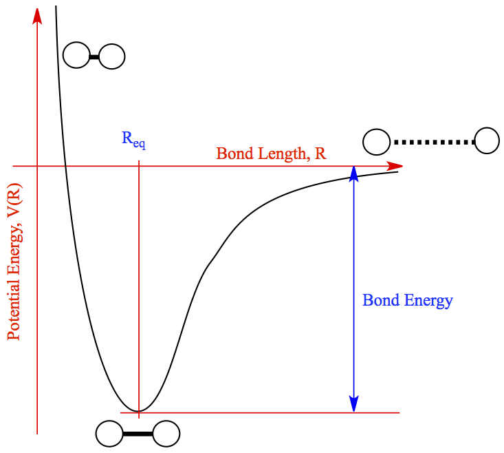
Each diatomic molecule has an equilibrium bond length that minimises its potential energy. If we increase the bond length beyond this equilibrium value, the two atoms that make up our dimer get further apart, so the negative attractive force between them becomes less negative, approaching zero at very large bond lengths. On the other hand, if we push the atoms closer together so that the bond length is less than the equilibrium value, the electrons will begin to repel each other via a positive repulsive force at very small bond lengths. Therefore, by varying the bond length for small distances around the equilibrium value, and calculating the energy using both classical and quantum methods, we should be able to observe a minimum in energy at the equilibrium bond length.
Tutorial notebook
The tutorial notebook is in folder exercise1 of the QTrain repository.
Notebook link: ICHEC/QTrain
Acknowledgements#
We extend our gratitude to the Irish Centre for High-End Computing (ICHEC) and University of Galway for providing computing and for all-encompassing invaluable support. This project was funded by the EuroHPC JU under grant agreement No 951732 and Ireland.

References#
ICHEC QPFAS repository
Hartree-Fock approximation
Sherrill, C. David. “An introduction to Hartree-Fock molecular orbital theory.” School of Chemistry and Biochemistry Georgia Institute of Technology https://vergil.chemistry.gatech.edu/static/content/hf-intro.pdf (2000).
Szabo, A., & Ostlund, N. S. (2012). Modern Quantum Chemistry: Introduction to Advanced Electronic Structure Theory. Courier Corporation.
Full Configuration Interaction
Helgaker, Trygve, Poul Jorgensen, and Jeppe Olsen. Molecular electronic-structure theory. John Wiley & Sons (2013).
VQE
https://learning.quantum.ibm.com/tutorial/variational-quantum-eigensolver
Peruzzo, Alberto, et al. “A variational eigenvalue solver on a photonic quantum processor.” Nature communications 5.1 https://www.nature.com/articles/ncomms5213 (2014).