Python For Quantum Mechanics#
Week 6: Scipy ODEs & PDEs#
from IPython.display import YouTubeVideo
YouTubeVideo('W6iLi9I90OM',width=700, height=400)
import matplotlib.pyplot as plt
from matplotlib import animation
from IPython.display import HTML


import numpy as np
import numpy.random as rnd

import scipy
from scipy import integrate
---------------------------------------------------------------------------
ModuleNotFoundError                       Traceback (most recent call last)
Cell In[2], line 9
      6 import numpy as np
      7 import numpy.random as rnd
----> 9 import scipy
     10 from scipy import integrate

ModuleNotFoundError: No module named 'scipy'
Integration#
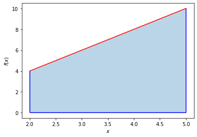
The function scipy.integrate.quad(f,a,b) integrates a function f(x) between the bounds [a,b] using a technique from the Fortran library QUADPACK and returns the value y of the definite integral integral and the error in this calculation,
$\(y = \int_a^b f(x)\ dx.\)$
def f(x):
    return 2*x
For example for the above function \(f(x) = 2x\) with the limits [\(2\),\(5\)] we get, $\(y = \int_2^5 \left(2x\right)\ dx = x^2 \bigg|_{x=2}^{x=5} = 5^2 - 2^2 = 21.\)$ The integral, of course, gives the area under the curve.
a = 2
b = 5

def_int, err = integrate.quad(f,a,b)

print('Area =',def_int)
print('Error =',err)

x = np.linspace(a,b,100)

fig = plt.figure()
ax = fig.add_axes([.1,.1,.8,.8])

ax.plot(x,f(x),'r')

ax.vlines([a,b],[0,0],[f(a),f(b)],'b')
ax.hlines(0,a,b,'b')
ax.fill_between(x,f(x),alpha=0.3)

ax.set_xlabel('$x$')
ax.set_ylabel('$f(x)$')

plt.show()
Area = 21.0
Error = 2.3314683517128287e-13
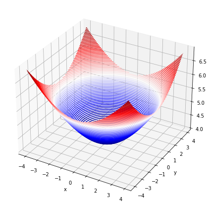
The function scipy.integrate.dblquad(g,a,b,c,d) integrates a function g(x,y) between the bounds [a,b] in x and [c,d] in y using a technique from the Fortran library QUADPACK and returns the value z of the definite integral integral and the error in this calculation,
$\(z = \int_c^d \int_a^b g(x,y)\ dx dy.\)$
def g(x,y):
    return np.sqrt(x**2 + y**2 +16)
a = -4
b = 4
c = -4
d = 4

def_int, err = integrate.dblquad(g,a,b,c,d)

print('Area =',def_int)
print('Error =',err)


x = np.arange(a,b,0.1)
y = np.arange(c,d,0.1)


Xmesh,Ymesh = np.meshgrid(x, y)
Zmesh = g(Xmesh,Ymesh)

fig = plt.figure(figsize=(7,7))
ax = fig.add_axes([.1,.1,.8,.8],projection='3d')

ax.contour3D(Xmesh,Ymesh,Zmesh,90,cmap='seismic')

ax.set_xlabel('x')
ax.set_ylabel('y')
plt.show()
Area = 327.8820544699914
Error = 4.38526073264293e-09
The function scipy.integrate.tplquad(h,a,b,c,d,e,f) integrates a function h(x,y,z) between the bounds [a,b] in x, [c,d] in y, and [e,f] in z using a technique from the Fortran library QUADPACK and returns the value k of the definite integral and the error in this calculation,
$\(k=\int_e^f \int_c^d \int_a^b h(x,y,z)\ dx dy dz.\)$
def h(x,y,z):
    return np.sqrt(x**2 + y**2 +z**2 +16)
lower_bound = -4
upper_bound = 4

def_int, err = integrate.tplquad(h,lower_bound,upper_bound,lower_bound,upper_bound,lower_bound,upper_bound)

print('Area = ',def_int)
print('Error = ',err)
Area =  2872.0630239126044
Error =  8.054480129954428e-09
Ordinary Differential Equations (ODEs)#
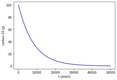
A first order ODE is an equation of the form $\(\frac{dy}{dt} = f(t,y). \)$ Lets do an example of radioactive decay, and how we can use scipy to solve an ode.
The half life of carbon-14 is 5700 years. It’s corrseponding decay constant is given by the formula $\(k = \frac{ln(\frac{1}{2})}{5700} = -0.0001216\)\( We can write an ordinary differential equation that encapsulates radioactive, exponential decay as follows \)\(\frac{dy}{dt} = k*y \)\( Lets solve this, for an initial \)100\(g sample of carbon-14, using `scipy.integrate.solve_ivp(fun, t_span, y0, method='RK45',t_eval=None)`. This solves an ODE, given an initial value `y0`, over a time span `t_span`, where the right hand side of the above equation is given by `fun`. The method of integration is set to fourth-order Runge-Kutta by default. `t_eval` can be set to an array that specifies the times at which to store the solution, otherwise this is set by default. The function returns multiple attributes, most importantly `.t` and `.y` which give the stored times and \)y$-values for the solution.
k = -0.0001216

def exponential_decay(t, y):
    return k * y

t = np.arange(0,50000,100)
sol = integrate.solve_ivp(exponential_decay, [0, 50000], [100], t_eval=t)

fig = plt.figure()
ax = fig.add_axes([.1,.1,.8,.8])

ax.plot(sol.t,sol.y[0,:],'b')
ax.set_xlabel('t (years)')
ax.set_ylabel('carbon-14 (g)')

plt.show()
We can also solve for multiple initial values of y, in other words that y0 can be an array. Here we have solution for \(100\)g, \(50\)g, and \(10\)g of carbon-14.
k = -0.0001216

def exponential_decay(t, y): return k * y

t = np.arange(0,50000,100)
sol = integrate.solve_ivp(exponential_decay, [0, 50000], [100,50,10], t_eval=t)

fig = plt.figure(figsize=(9,6))
ax = fig.add_axes([.1,.1,.8,.8])

ax.plot(sol.t,sol.y[0,:],'b',label = '$100$g')
ax.plot(sol.t,sol.y[1,:],'r',label = '$50$g')
ax.plot(sol.t,sol.y[2,:],'g',label = '$10$g')

ax.set_xlabel('t (years)')
ax.set_ylabel('carbon-14 (g)')

plt.show()

Finite-Difference Method#
Taylor’s Theorem#
The taylor series allows us to approximate derivatives, particularly in a discrete step-wise manner. We will leverage this to our advantage, greatly simplifying integral and derivative problems.
Lets start by truncating the series at \(n=1\), assuming that the remainder \(R_1(x)\) can be neglected.
Thus we have an approximation for the first derivative over a discrete step \(h\).
The Laplace Operator#
Lets do the something similar for the second derivative
Adding these two equations gives
This is known as the Central-Difference Approximation.
Suppose we have six discrete values of a function \(f\) inside some array/vector
We can transform this vector, multiplying by some matrix, that finds the second derivative at each discrete point \(f_i\) using the above approximation.
Where \(h\) is the spacing between discrete inputs to \(f\).
We will call this matrix/operator the Laplace Operator and label it as \(\textbf{L}\), so that for \(n\) discrete values of a function
Notice, that we can classify this as a sparse matrix, and leverage this using scipy.
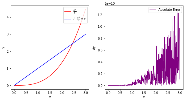
Lets test this on \(\frac{x^3}{6}\), where \(\frac{d^2}{dx^2}\frac{x^3}{6}=x\)
h = 0.005
x = np.arange(0, 3, h)
size = x.size

L = scipy.sparse.diags([1, -2, 1],[-1, 0, 1],shape=(size,size))/h**2

Error = abs(x[1:-1]-L.dot((x**3)/6)[1:-1])

fig = plt.figure(figsize=(10,5))
ax1 = plt.subplot(121)
ax2 = plt.subplot(122)

ax1.plot(x[1:-1], ((x**3)/6)[1:-1], label=r"$\frac{x^3}{6}$",color="red")
ax1.plot(x[1:-1], L.dot(((x**3)/6))[1:-1], label=r"$L \cdot \frac{x^3}{6} = x$",color="blue")
ax1.legend(loc=1)
ax1.set_xlabel('x')
ax1.set_ylabel('y')


ax2.plot(x[1:-1],Error,label="Absolute Error",color="purple")
ax2.legend(loc=1)
ax2.set_xlabel('x')
ax2.set_ylabel(r"$\Delta y$")

plt.show()
Partial Differential Equations (PDEs)#
The Schrödinger Equation#
Lets use the above function to solve a PDE, namely the time-independent Schrödinger equation in one-dimension: $\(\frac{-\hbar^2}{2m}\frac{\partial{}^2}{\partial{x^2}}\psi(t,x) + V(x)\psi(t,x) = i\hbar \frac{\partial{}}{\partial{t}}\psi(t,x) \)$
We can rewrite this equation in the following way $\(i\hbar\frac{\partial{}}{\partial{t}}\psi(t,i) = \left[\frac{-\hbar^2}{2m}\textbf{L} + V(i)\right]\psi(t,i) \)\( Where \)x\rightarrow i$ is interpreted as discretising the problem. We have thus reduced the problem to an ODE, as seen above.
Let’s investigate, and solve the problem, with various potentials \(V(x)\).
The Quantum Harmonic Osciallator#
Where \(\omega\) is the angular frequency of the oscillator, and \(T\) is it’s period, \(m\) is the mass. \(a\) is the centre of oscialltion.
For ease, \(m=\hbar=T=1 \implies \omega = 2\pi\) and
#Initialise the discrete spatial points, x, into an array
h = 0.005
x = np.arange(-10, 10, h)
size = x.size

#Define the Laplace Operator
L = scipy.sparse.diags([1, -2, 1], [-1, 0, 1], shape=(size, size)) / h**2

#Initialise the parameter values and potential V
hbar = 1
m = 1
w = 2*np.pi
a = 0
V = 0.5*m*(w**2)*(x-a)**2

#Define the function to be integrated
def wave_fun(t, psi):
    return -1j*(-(hbar/(2*m))*L.dot(psi) + (V/hbar)*psi)

# Time range for integration
t_eval = np.arange(0.0, 1.0, h)
We will define our initial state \(\psi(t=0)\) as that of a wave packet scene in the previous section 6.4
Where \(\sigma\) is the width, \(x_0\) is it’s position, and \(f\) is it’s frequency.
#Defining the initial state psi
f = 8*(2*np.pi)
sigma = 1.0
x0 = a
packet = (1.0/np.sqrt(sigma*np.sqrt(np.pi)))*np.exp(-(x-x0)**2/(2.0*sigma**2))*np.exp(1j*f*x)

#Normalise
packet = packet/(np.sqrt(sum((abs(packet))**2)))
We will now solve using
scipy.integrate.solve_ivp(fun, t_span, y0, method='RK45',t_eval=None)
sol = integrate.solve_ivp(wave_fun, t_span = [0, 1], y0 = packet, t_eval = t_eval)
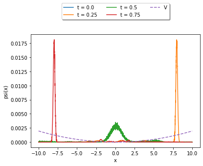
Now lets plot
#Plot the result at different times
fig = plt.figure()
ax = fig.add_axes([.1,.1,.8,.8])

for i, t in enumerate(sol.t):
    if i%50==0:
        ax.plot(x, np.abs(sol.y[:,i])**2,label='t = {}'.format(t))

#Plot the potential, adjusting size for visual aid
ax.plot(x, V*0.000001, "--", label='V')

ax.legend(loc='upper center', bbox_to_anchor=(0.5, 1.3), ncol=3, fancybox=True, shadow=True)

ax.set_xlabel('x')
ax.set_ylabel('psi(x)')
plt.show()
%matplotlib notebook

fig = plt.figure()
ax1 = fig.add_axes([.1,.1,.8,.8])

ax1.set_xlim(-10, 10)
ax1.set_ylim(-0.1, 0.1)
ax1.set_xlabel('x')
ax1.set_ylabel('psi(x)')

title = ax1.set_title('The Quantum Harmonic Osciallator')

line1, = ax1.plot([], [], "--")
line2, = ax1.plot([], [],color='red')


def init():
    line1.set_data(x, V*0.000001)
    return line1,


def animate(i):
    line2.set_data(x, sol.y[:,i])
    title.set_text('t = {0:1.3f}'.format(sol.t[i]))
    return line1,


anim = animation.FuncAnimation(fig, animate, init_func=init, frames=len(sol.t), interval=50, blit=True)

plt.show()

Fourier Transform#
from numpy.fft import fftfreq
from scipy import fftpack


F = fftpack.fft(sol.y[:,0])
w = fftfreq(size, h)
F = F/(np.sqrt(sum((abs(F))**2)))

indices = w > 0 # select only indices for elements that corresponds to positive frequencies
w_pos = w[indices]
F_pos = F[indices]

fig, ax = plt.subplots(figsize=(9,3))
ax.plot(w_pos, abs(F_pos))
ax.set_xlim(0, 10);

F = np.zeros(shape=(size,sol.y.size),dtype='complex')
w = fftfreq(size, h)


for i, t in enumerate(sol.t):
    F[:,i] = fftpack.fft(sol.y[:,i])
    F[:,i] = F[:,i]/(np.sqrt(sum((abs(F[:,i])**2))))
    sol.y[:,i] = sol.y[:,i]/(np.sqrt(sum((abs(sol.y[:,i])**2))))

print(np.sqrt(sum((abs(F[:,i])**2))))
print(np.sqrt(sum((abs(sol.y[:,i])**2))))
1.0000000000000013
0.999999999999998
print(max(sol.y[:,0])/max(F[:,0]).real)
%matplotlib notebook
fig, (ax1,ax2) = plt.subplots(2,1)

limit = 2.5*max(F[:,0])
scaler = 1/(max(V)/limit)

ax1.set_xlim(x[0], x[-1])
ax1.set_ylim(-limit,limit)
ax1.set_xlabel('$x$')
ax1.set_ylabel('$\psi(x)$')

ax2.set_xlim(x[0], x[-1])
ax2.set_ylim(-limit, limit)
ax2.set_xlabel('$w=p/h$')
ax2.set_ylabel('$\psi(w)$')

title = ax1.set_title('The Quantum Harmonic Osciallator')

line1, = ax1.plot([], [], ls="--")
line2, = ax1.plot([], [],color='red', lw=.2)
line3, = ax2.plot([], [],color='blue', lw=.2)
line4, = ax2.plot([], [], ls="--")

def init():
    line1.set_data(x, V*scaler)
    line4.set_data(x, V*scaler)
    return line1,line4


def animate(i):
    line2.set_data(x, sol.y[:,i])
    line3.set_data(w, F[:,i])
    title.set_text('$t = {0:1.3f}$'.format(sol.t[i]))
    return line2,line3

anim = animation.FuncAnimation(fig, animate, init_func=init, frames=len(sol.t), interval=50, blit=True)
plt.show()
(0.12615662610102787+9.912719241054443e-12j)

Step Potential & Quantum Tunnelling#
h = 0.005
x = np.arange(0, 10, h)
size = x.size

LO = scipy.sparse.diags([1, -2, 1], [-1, 0, 1], shape=(size, size)) / h**2

hbar = 1
m=1

x_Vmin = 5         # center of V(x)
T      = 1

omega = 2 * np.pi / T
k = omega**2 * m
V = np.zeros(size)
V[int(V.size/2):] = x_Vmin*250

def psi_t(t, psi):
    return -1j * (- 0.5 * hbar / m * LO.dot(psi) + V / hbar * psi)

dt = 0.001  # time interval for snapshots
t0 = 0.0    # initial time
tf = 0.2   # final time
t_eval = np.arange(t0, tf, dt)  # recorded time shots

sigma=0.5
x0 = 3.0
kx = 50
A = 1.0 / (sigma * np.sqrt(np.pi))
psi0 = np.sqrt(A) * np.exp(-(x-x0)**2 / (2.0 * sigma**2)) * np.exp(1j * kx * x)


# Solve the Initial Value Problem
sol = integrate.solve_ivp(psi_t, t_span = [t0, tf], y0 = psi0, t_eval = t_eval)
%matplotlib notebook

fig = plt.figure()
ax1 = plt.subplot(1,1,1)
ax1.set_xlim(0, 10)
ax1.set_ylim(-6, 6)
title = ax1.set_title('')
line1, = ax1.plot([], [], "k--")
line2, = ax1.plot([], [])


def init():
    line1.set_data(x, V * 0.001)
    return line1,


def animate(i):
    line2.set_data(x, (sol.y[:,i]).real)
    title.set_text('Time = {0:1.3f}'.format(sol.t[i]))
    return line1,


anim = animation.FuncAnimation(fig, animate, init_func=init,
                               frames=len(sol.t), interval=50, blit=True)
plt.show()

%matplotlib notebook

fig = plt.figure()
ax1 = plt.subplot(1,1,1)
ax1.set_xlim(0, 10)
ax1.set_ylim(-6, 6)
title = ax1.set_title('')
line1, = ax1.plot([], [], "k--")
line2, = ax1.plot([], [])


def init():
    line1.set_data(x, V * 0.001)
    return line1,


def animate(i):
    line2.set_data(x, (np.abs(sol.y[:,i]))**2)
    title.set_text('Time = {0:1.3f}'.format(sol.t[i]))
    return line1,


anim = animation.FuncAnimation(fig, animate, init_func=init,
                               frames=len(sol.t), interval=50, blit=True)
plt.show()

F = fftpack.fft(sol.y[:,0])
w = fftfreq(size, h)

indices = w > 0 # select only indices for elements that corresponds to positive frequencies
w_pos = w[indices]
F_pos = F[indices]

fig, ax = plt.subplots(figsize=(9,3))
ax.plot(w_pos, abs(F_pos))
ax.set_xlim(0, 10)

plt.show()
