Python For Quantum Mechanics#
Week 6: Scipy Optimization#
from IPython.display import YouTubeVideo
YouTubeVideo('p2ohSsd1KTg',width=700, height=400)
import matplotlib.pyplot as plt
import numpy as np
import numpy.random as rnd
import scipy
from scipy import optimize
---------------------------------------------------------------------------
ModuleNotFoundError                       Traceback (most recent call last)
Cell In[2], line 4
      2 import numpy as np
      3 import numpy.random as rnd
----> 4 import scipy
      5 from scipy import optimize

ModuleNotFoundError: No module named 'scipy'
Function Minimum#
def f(b):
    return -(.6*np.log(1+b[0]-b[1]-b[2])+.3*np.log(1-b[0]+2*b[1]-b[2])+.1*np.log(1-b[0]-b[1]+4*b[2]))
from scipy.optimize import Bounds
bounds = Bounds([0.0, 1.0], [0.0, 1.0],[0.0, 1.0])

initial_guess = np.array([0.0,0.0,0.0])
result = optimize.minimize(f, initial_guess, bounds=bounds)
print(result)
---------------------------------------------------------------------------
IndexError                                Traceback (most recent call last)
Input In [23], in <cell line: 4>()
      2 bounds = Bounds([0.0, 1.0], [0.0, 1.0],[0.0, 1.0])
      3 initial_guess = np.array([0.0,0.0,0.0])
----> 4 result = optimize.minimize(f, initial_guess, bounds=bounds)
      5 print(result)

File /usr/local/lib/python3.9/site-packages/scipy/optimize/_minimize.py:643, in minimize(fun, x0, args, method, jac, hess, hessp, bounds, constraints, tol, callback, options)
    638 i_fixed = (bounds.lb == bounds.ub)
    640 if np.all(i_fixed):
    641     # all the parameters are fixed, a minimizer is not able to do
    642     # anything
--> 643     return _optimize_result_for_equal_bounds(
    644         fun, bounds, meth, args=args, constraints=constraints
    645     )
    647 # determine whether finite differences are needed for any grad/jac
    648 fd_needed = (not callable(jac))

File /usr/local/lib/python3.9/site-packages/scipy/optimize/_minimize.py:1007, in _optimize_result_for_equal_bounds(fun, bounds, method, args, constraints)
   1001         success = False
   1002         message = (f"All independent variables were fixed by bounds, but "
   1003                    f"the independent variables do not satisfy the "
   1004                    f"constraints exactly. (Maximum violation: {maxcv}).")
   1006 return OptimizeResult(
-> 1007     x=x0, fun=fun(x0, *args), success=success, message=message, nfev=1,
   1008     njev=0, nhev=0,
   1009 )

Input In [10], in f(b)
      1 def f(b):
----> 2     return -(.6*np.log(1+b[0]-b[1]-b[2])+.3*np.log(1-b[0]+2*b[1]-b[2])+.1*np.log(1-b[0]-b[1]+4*b[2]))

IndexError: index 2 is out of bounds for axis 0 with size 2
Given some function we are able to find a local minimum using scipy.optimize.fmin(f,x0), where f is the function in question, x0 is an initial guess.
def f(x):
    return x**4 + x**3 + x**2 - 7*x + 10
x = np.linspace(-3,3,100)

y = f(x)

fig = plt.figure()
ax = fig.add_axes([.1,.1,.8,.8])

ax.plot(x,y)

plt.show()
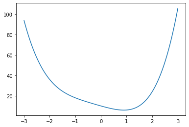
x_min = optimize.fmin(f, 0)
print(x_min)
Optimization terminated successfully.
         Current function value: 5.894475
         Iterations: 24
         Function evaluations: 48
[0.8914375]
However if the function has multiple local minima the initial guess will determine which is found.
def g(x):
    return x**4 - x**3 - 5* x**2 + x + 0
x = np.linspace(-2,3,100)

y = g(x)

fig = plt.figure()
ax = fig.add_axes([.1,.1,.8,.8])

ax.plot(x,y)

plt.show()
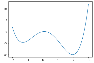
x_min1 = optimize.fmin(g, -1)
print('x_min1 =',x_min1,'\n')

x_min2 = optimize.fmin(g, 1)
print('x_min2 =',x_min2)
Optimization terminated successfully.
         Current function value: -4.697455
         Iterations: 14
         Function evaluations: 28
x_min1 = [-1.3078125]

Optimization terminated successfully.
         Current function value: -10.019646
         Iterations: 16
         Function evaluations: 32
x_min2 = [1.96025391]
Global Optimization#
We can find the global minimum of a function, within given bounds, using scipy.optimize.differential_evolution(func,bounds). bounds will be a list of lists containing the max and min of the input parameters of func. It should be noted that this works best when func takes in one argument which is a list of the input parameters. Running this function returns the information about the optomisation process with the min value found stored as x.
result = scipy.optimize.differential_evolution(g,[[-2,3]])

print(result)
     fun: array([-10.01964635])
     jac: array([-1.42108548e-06])
 message: 'Optimization terminated successfully.'
    nfev: 68
     nit: 3
 success: True
       x: array([1.96027333])
A similar process can be achieved with multivariable functions too.
def f(params):
    return -100. * np.exp(-0.1*np.sqrt(params[0]**2 + params[1]**2)) + np.exp(np.cos(params[0]) + np.cos(params[1]))

x_bound = [-20,20]
y_bound = [-20,20]

xs = np.linspace(x_bound[0], x_bound[1], 100)
ys = np.linspace(y_bound[0], y_bound[1], 100)

Xmesh,Ymesh = np.meshgrid(xs, ys)
Zmesh = f([Xmesh,Ymesh])

fig = plt.figure(figsize=(7,7))
ax = fig.add_axes([.1,.1,.8,.8],projection='3d')

ax.contour3D(Xmesh,Ymesh,Zmesh,90,cmap='seismic')

plt.show()
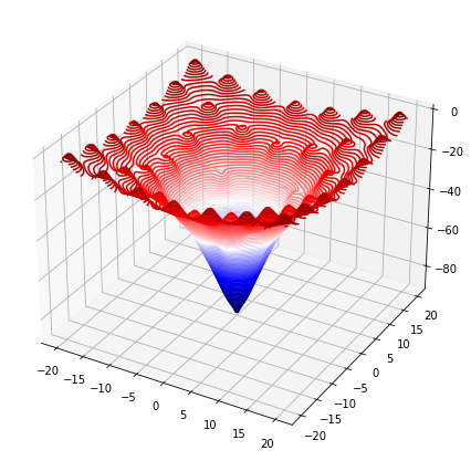
bounds = [x_bound,y_bound]
result = scipy.optimize.differential_evolution(f,bounds)

print(np.round(result.x,2))
[-0. -0.]
Function Roots#
The function scipy.optimize.fsolve(f,x0) finds the roots of a function f, given an initial guess array x0.
randy = rnd.random(3)

def f(x):
    return 0.25*randy[0]*x**2 - randy[1]*2*x - randy[2]
x = np.linspace(-20,40,100)

y = f(x)

y2 = np.zeros(len(x))

fig = plt.figure()
ax = fig.add_axes([.1,.1,.8,.8])
ax.set_xlim(x[0],x[-1])

ax.plot(x,y,x,y2)

plt.show()
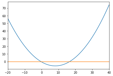
roots = optimize.fsolve(f,[x[0],x[-1]])

print(roots)

print(np.round(f(roots),2))
[-0.37906637 16.59148356]
[-0.  0.]
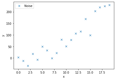
Optimize Least Square Fit#
Lets try and fit a curve to the following noisy data.
c1, c2 = 0.5, 2.0

x = np.arange(20)

y = c1*x**2 + c2*x

noise = y + 0.2 * np.max(y) * rnd.random(len(y))*((-1)**(2-(np.round(rnd.random(len(y)),0))))

fig = plt.figure()
ax = fig.add_axes([.1,.1,.8,.8])

ax.plot(x,noise,'x',label='Noise')
ax.set_xlabel('x')
ax.set_ylabel('y')
ax.legend()

plt.show()
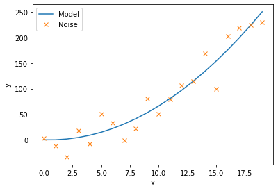
We will now define a function to model this curve, as well as a function that calculates the residuals. The residuals are the differrence between each noisy data point and the model being fitted. This scipy.optimize.leastsq(residuals,c_guess, args=(noise,x)) function gives back the coefficient c that minimises the residuals. We must input the noisy data, noise, and their corresponding x co-ordinates, as well as an intial guess for the coefficients c_guess.
def model(x, c):
    return c[0]*x**2 + c[1]*x

def residuals(c,y,x):
    return y - model(x,c)

c_guess = np.array([0.0,2.1])

c_result, flag = scipy.optimize.leastsq(residuals,c_guess, args=(noise,x))

print(c_result)

fig = plt.figure()
ax = fig.add_axes([.1,.1,.8,.8])

ax.plot(x, model(x,c_result), label='Model')
ax.plot(x, noise, 'x', label='Noise')
ax.set_xlabel('x')
ax.set_ylabel('y')
ax.legend()

plt.show()
[ 0.7283107 -0.65686655]
Curve Fit#
The scipy.optimize.curve_fit(model,xdata,ydata,p0) function allows us to directly input the model function aswell the noisy data, (xdata,ydata), along with an initial guess for the model coefficients p0. We must define our model function with indiviual coefficeients rather than an array of cefficients.
def model(x, c1, c2):
    return c1*x**2 + c2*x

c_result, flag = scipy.optimize.curve_fit(model,x,noise,p0=(0.5,2.0))

print(c_result)

fig = plt.figure()
ax = fig.add_axes([.1,.1,.8,.8])

ax.plot(x,model(x,c_result[0],c_result[1]),label='Model')
ax.plot(x,noise,'x',label='Noise')
ax.set_xlabel('x')
ax.set_ylabel('y')
ax.legend()

plt.show()
[ 0.72831071 -0.65686659]