Python for Quantum Mechanics:#
3D Plots and Animations#
from IPython.display import YouTubeVideo
YouTubeVideo('2GGQqxRI3fs',width=700, height=400)
import numpy as np
import matplotlib.pyplot as plt
Line Plot#
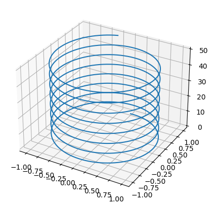
To make a 3D plot you must first create a set of axes with the keyword projection set to '3d'. Then we can populate it with a line using the .plot3D() attribute function of the axes object. This is similar to plt.plot(), only now it will have three instead of two array argumanets.
fig = plt.figure()
ax = fig.add_axes([0.1,0.1,.8,.8], projection='3d')

z = np.arange(0, 50, .01)
x_spiral, y_spiral = np.sin(z), np.cos(z)

ax.plot3D(x_spiral, y_spiral, z)
#ax.view_init(60, 35)

plt.show()
Heat Map#
For plotting a surface it is best to create a 2D mesh grid of points using np.meshgrid(); this takes in two numpy arrays that can be thought of as \(x\) and \(y\) axes to this grid. Lets say the arrays are of lengths \(m\) and \(n\). The function creates two \(n \times m\) matrices; one with rows eqaul to the \(x\)-array and one with the columns equal to \(y\)-array.
xs = np.linspace(0, 10, 5)
ys = np.linspace(-5, 5, 11)

Xmesh,Ymesh = np.meshgrid(xs, ys)
print('xs =', xs, '\n')
print('Xmesh =', Xmesh, '\n')
print('ys =', ys, '\n')
print('Ymesh =', Ymesh)
xs = [ 0.   2.5  5.   7.5 10. ]

Xmesh = [[ 0.   2.5  5.   7.5 10. ]
 [ 0.   2.5  5.   7.5 10. ]
 [ 0.   2.5  5.   7.5 10. ]
 [ 0.   2.5  5.   7.5 10. ]
 [ 0.   2.5  5.   7.5 10. ]
 [ 0.   2.5  5.   7.5 10. ]
 [ 0.   2.5  5.   7.5 10. ]
 [ 0.   2.5  5.   7.5 10. ]
 [ 0.   2.5  5.   7.5 10. ]
 [ 0.   2.5  5.   7.5 10. ]
 [ 0.   2.5  5.   7.5 10. ]]

ys = [-5. -4. -3. -2. -1.  0.  1.  2.  3.  4.  5.]

Ymesh = [[-5. -5. -5. -5. -5.]
 [-4. -4. -4. -4. -4.]
 [-3. -3. -3. -3. -3.]
 [-2. -2. -2. -2. -2.]
 [-1. -1. -1. -1. -1.]
 [ 0.  0.  0.  0.  0.]
 [ 1.  1.  1.  1.  1.]
 [ 2.  2.  2.  2.  2.]
 [ 3.  3.  3.  3.  3.]
 [ 4.  4.  4.  4.  4.]
 [ 5.  5.  5.  5.  5.]]
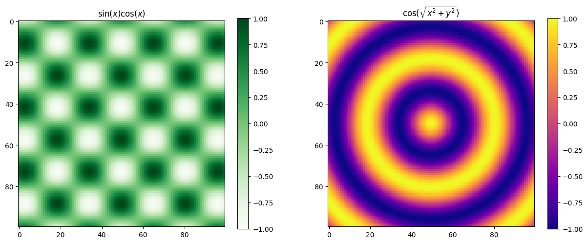
This can can then be used to sample a a grid of \(x\)- and \(y\)-axes. We can use these to give each of the grid points a value and plot this. The plt.pcolormesh() can be easily used to create a colour projection of a 3d plot. A colour map (cmap keyword) is used to specify what colours are mapped to by each value.
def f(x, y):
    return np.cos(np.sqrt(x**2 +y**2))

def g(x, y):
    return np.cos(x) * np.sin(y)
xs = np.linspace(-10, 10, 100)
ys = np.linspace(-10, 10, 100)

Xmesh,Ymesh = np.meshgrid(xs, ys)
Zmesh0 = g(Xmesh,Ymesh)
Zmesh1 = f(Xmesh,Ymesh)

fig, ax = plt.subplots(1,2, figsize=(15,10))

im0 = ax[0].imshow(Zmesh0, cmap = 'Greens')
im1 = ax[1].imshow(Zmesh1, cmap = 'plasma')
fig.colorbar(im0, ax=ax[0], shrink = .56)
fig.colorbar(im1, ax=ax[1], shrink = .56)

ax[0].set_title('$\sin (x) \cos (x)$')
ax[1].set_title('$\cos ( \sqrt{x^2 +y^2} )$')

im0.set_clim([-1,1])
im1.set_clim([-1,1])

plt.show()
<>:15: SyntaxWarning: invalid escape sequence '\s'
<>:16: SyntaxWarning: invalid escape sequence '\c'
<>:15: SyntaxWarning: invalid escape sequence '\s'
<>:16: SyntaxWarning: invalid escape sequence '\c'
/tmp/ipykernel_2612/3047540586.py:15: SyntaxWarning: invalid escape sequence '\s'
  ax[0].set_title('$\sin (x) \cos (x)$')
/tmp/ipykernel_2612/3047540586.py:16: SyntaxWarning: invalid escape sequence '\c'
  ax[1].set_title('$\cos ( \sqrt{x^2 +y^2} )$')
Plotting a Surface#
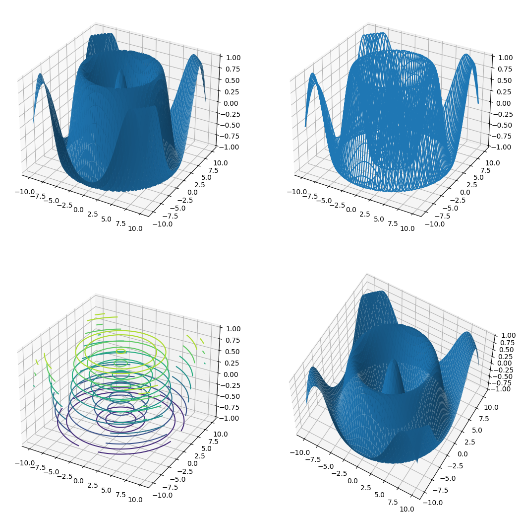
A surface can be plotted in different ways using .plot_surface(), .plot_wireframe(), or .contour3D() attribute function. We can change the view angle on the plot using .view_init() by specifying the azimuthal angle azim and the angle of elevation elev in degrees.
xs = np.linspace(-10, 10, 100)
ys = np.linspace(-10, 10, 100)

Xmesh,Ymesh = np.meshgrid(xs, ys)
Zmesh = f(Xmesh,Ymesh)

fig = plt.figure(figsize=(13,13))

ax1 = fig.add_subplot(2, 2, 1, projection='3d')
ax2 = fig.add_subplot(2, 2, 2, projection='3d')
ax3 = fig.add_subplot(2, 2, 3, projection='3d')
ax4 = fig.add_subplot(2, 2, 4, projection='3d')


ax1.plot_surface(Xmesh,Ymesh,Zmesh)
ax2.plot_wireframe(Xmesh,Ymesh,Zmesh)
ax3.contour3D(Xmesh,Ymesh,Zmesh)
ax4.plot_surface(Xmesh,Ymesh,Zmesh)
ax4.view_init(azim=-60, elev=60)

plt.show()
Interactive Backend#
In IPython there exists a magic function, %matplotlib, that allows the us to specify the backend for matplotlib. So far we have only been using the default %matplotlib inline. For some applictaions it can be useful to use %matplotlib notebook which allows interactivity and evolution in time. You always need to be mindful to ‘turn off’ the image when you are done interacting with it.
%matplotlib notebook

import numpy as np
import matplotlib.pyplot as plt
We can mess around the the below image.
fig = plt.figure()
ax = fig.add_axes([0.1,0.1,.8,.8])

x = np.arange(.1,10,.001)
y1 = 1/x + 3*np.sin(x*100)

ax.plot(x,y1)
ax.set_xlim(2, 4)

plt.show()
y2 = 1/x + 3*np.cos(x*100)

ax.plot(x,y2)

plt.show()
Animations#
To do animations we need a function, FuncAnimation().
from matplotlib.animation import FuncAnimation
This function takes in a number of arguments that are required.
We need a figure fig, that needs animating with an axis ax. We will do the usual setup.
fig_anim = plt.figure()
ax_anim = fig_anim.add_axes([.1,.1,.8,.8])

ax_anim.set_xlim(0, 2)
ax_anim.set_ylim(-2, 2)
ax_anim.grid()

plt.show()
Now keeping this active we will add a plot to the picture. Notice that when we plot we have saved the return line item. The , is present because this is in ax.plot() will in fact return a tupple with the needed item as the first item.
ax_anim.set_xlim(0, 2)
ax_anim.set_ylim(-2, 2)

line, = ax_anim.plot([], [])

plt.show()
The FuncAnimation() function requires an initialise function (the init_func keyword will be used) that will be called at the start of the animation. We will use the .set_data() which gives the data for the curve in the form of two arrays.
def init():
    x = np.linspace(0, 2, 1000)
    y = np.sin(2 * np.pi * x)
    line.set_data(x, y)
    return line,
We will also need to define an other function that will be called repeatedly. This will change the data in our plot in each successive calling of the function.
def animate(i):
    x = np.linspace(0, 2, 1000)
    y = np.sin(2 * np.pi * (x - 0.01 * i))
    line.set_data(x, y)
    return line,
The FuncAnimation() can now be called with added keywords
frames: Number of frames long animation will be.interval: number of milliseconds inbetween frames.repeat_delay:blit: IfTruewill not replot parts of lines that are already plotted so it will animate faster.
anim = FuncAnimation(fig_anim, animate, init_func=init, frames=100, interval=20, repeat_delay=300, blit=True)

plt.show()
To save an animation we need a writer. We will import matplotlib.animation.PillowWriter() to do this.
from matplotlib.animation import PillowWriter

mywriter = PillowWriter(fps = 30)
Finally we save the animation.
anim.save('my_animation.gif', writer = mywriter)