Sage Notebook#
This is an introductory tutorial. Knowledge of python is going to be very handy.
The simplest thing you can do with sage is some arithmatic! However, you have access to several function for basic number functions.
x = 2+3
print(x)
5
is_prime(x)
# get a list of primes
N = 1000
list_primes = [i for i in [2..N] if is_prime(i)]
print(list_primes)
[2, 3, 5, 7, 11, 13, 17, 19, 23, 29, 31, 37, 41, 43, 47, 53, 59, 61, 67, 71, 73, 79, 83, 89, 97, 101, 103, 107, 109, 113, 127, 131, 137, 139, 149, 151, 157, 163, 167, 173, 179, 181, 191, 193, 197, 199, 211, 223, 227, 229, 233, 239, 241, 251, 257, 263, 269, 271, 277, 281, 283, 293, 307, 311, 313, 317, 331, 337, 347, 349, 353, 359, 367, 373, 379, 383, 389, 397, 401, 409, 419, 421, 431, 433, 439, 443, 449, 457, 461, 463, 467, 479, 487, 491, 499, 503, 509, 521, 523, 541, 547, 557, 563, 569, 571, 577, 587, 593, 599, 601, 607, 613, 617, 619, 631, 641, 643, 647, 653, 659, 661, 673, 677, 683, 691, 701, 709, 719, 727, 733, 739, 743, 751, 757, 761, 769, 773, 787, 797, 809, 811, 821, 823, 827, 829, 839, 853, 857, 859, 863, 877, 881, 883, 887, 907, 911, 919, 929, 937, 941, 947, 953, 967, 971, 977, 983, 991, 997]
It starts to become more interesting, when you notice that sage is a computer algebra system!
You can do symbolic manipulations.
f(x) = x^2
g(x) = sin(f(x))^3
show(
derivative(g(x), x)
)
\(\displaystyle 6 \, x \cos\left(x^{2}\right) \sin\left(x^{2}\right)^{2}\)
show(
integral(derivative(g(x), x), x)
)
show(
integral(f(x), x)
)
show(
integral(sqrt(x^2-4), x)
)
\(\displaystyle \sin\left(x^{2}\right)^{3}\)
\(\displaystyle \frac{1}{3} \, x^{3}\)
\(\displaystyle \frac{1}{2} \, \sqrt{x^{2} - 4} x - 2 \, \log\left(2 \, x + 2 \, \sqrt{x^{2} - 4}\right)\)
z = (1+x)^9
show(
z.expand()
)
\(\displaystyle x^{9} + 9 \, x^{8} + 36 \, x^{7} + 84 \, x^{6} + 126 \, x^{5} + 126 \, x^{4} + 84 \, x^{3} + 36 \, x^{2} + 9 \, x + 1\)
y = z.expand()
show(
y.factor()
)
\(\displaystyle {\left(x + 1\right)}^{9}\)
Plotting#
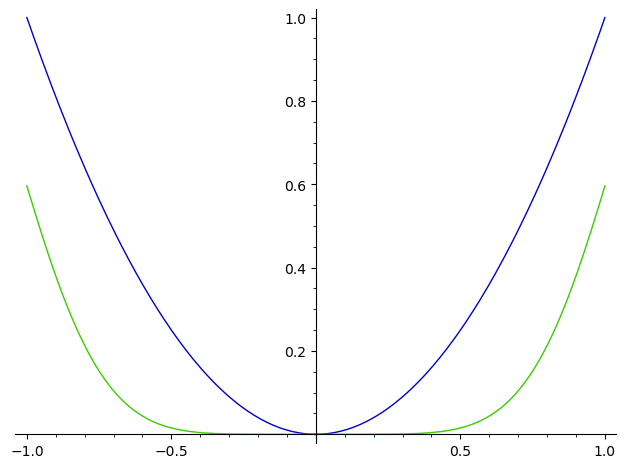
One can plot functions
plot([f, g], (x, -1, 1))
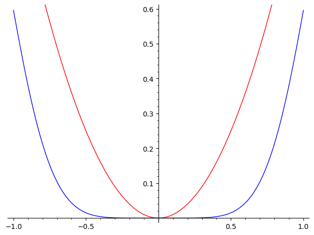
# You can save graph as object to manipulate later.
F = plot(f, (x, -1, 1), color='red')
G = plot(g, (x, -1, 1), color='blue')
# some plotting constraints can be passed to .show() method
(F+G).show(ymax=0.6)
h(x, y) = sin(x^2 + y^2)
plot3d(h, (x, -5, 5), (y, -5, 5))
var('x,y,z')
T = golden_ratio
p = 2 - (cos(x + T*y) + cos(x - T*y) + cos(y + T*z) + cos(y - T*z) + cos(z - T*x) + cos(z + T*x))
r = 4.78
implicit_plot3d(p, (x, -r, r), (y, -r, r), (z, -r, r), plot_points=50, color='yellow')
Number theory examples#
K.<a> = NumberField(x^2-1000003)
K.units()
(13588539824738670501937634049552988333821695209017845709174282597854911795746277767704092880505583734383723377832872303678298905016746850960859455536870699535559837726582129371990014046340205582554652629926918221158254563735625476440662077676454369*a + 13588560207533120525571173911036889359175071334492475577050945981112655754066115844008109262853595087091825489817727423098897434120714422347327176783787901807748239401349778788112430877903180798732552113299179825446080855972862801189963185573195143522,)
K.class_number()
3
log(3).n()
1.09861228866811